STA410 Assignment 2
Michal Malyska
2018-10-16
library(tidyverse)
set.seed(271828)
knitr::opts_chunk$set(cache = TRUE)
#Question 1
##a)
It is enough to show that the inverse CDF has a closed from, and then we can just plug in the randomly generated unifrom(0,1) to get the distribution as mentioned in the inverse method alogrithms.
\[ \int g(x;s) = G(x;s) = \frac{1}{1+e^{\frac{x}{s}}} \]
\[G(x;s) = \frac{1}{1+e^{-\frac{x}{s}}} \Rightarrow\] \[\Rightarrow G^{-1}(x;s) = (\frac{1}{1+e^{-\frac{x}{s}}})^{-1} \Leftrightarrow\] \[ \Leftrightarrow \frac{1}{G^{-1}(x;s)} - 1 = \exp{\left( -\frac{x}{s} \right)} \Leftrightarrow\] \[ \Leftrightarrow X = s \log \left( \frac{G^{-1}(x;s)}{1+G^{-1}(x;s)} \right)\] Now we plug in the U as \(G^{-1}(x;s)\) to get:
\[ X = s \log \left( \frac{U}{1+U} \right) \]
##b)
In this part of the question, consider the region \(s \geq \frac{1}{\sqrt{2}}\).
We approach the problem by minimizing the log of \(M(s)\) since log is monotone.
\[\max_x M(s,x) = \frac{f(x)}{g(x;s)} \Rightarrow \max \log M(s,x) = \log f(x) - \log g(x;s) \]
We plug in the definition of each function and simplify in order to obtain:
\[ \log M(s,x) = -\frac{x^2}{s} - \frac{x}{s} + 2 \log( 1 + e^{ \left(\frac{x}{s} \right)} ) \Rightarrow\]
\[ \Rightarrow \frac{d}{dx}\log M(s,x) = -x - \frac{1}{s} + \frac{2 e^{ \left(\frac{x}{s} \right) }}{s (1 + e^{ \left(\frac{x}{s} \right)})} \Rightarrow \]
\[\frac{d^2}{dx^2}\log M(s,x) = -1 + \frac{2}{s}\frac{\frac{1}{s} e^{ \left(\frac{x}{s} \right)}(1 + e^{ \left(\frac{x}{s} \right)}) - \frac{1}{2} (e^{ \left(\frac{x}{s} \right)})^2}{(1+ e^ {\left(\frac{x}{s} \right)})^2} \]
Now evaluate the derivative at \(x=0\) and see that:
\[ \frac{d}{dx}\log M(s) \mid_{x=0} = 0 \]
Hence \(x=0\) is a critical value. Evaluating the second derivative at the same point we get that:
\[ \frac{d^2}{dx^2}\log M(s) \mid_{x=0} = 1- \frac{1}{2s^2} \]
This is positive for \(s \geq \frac{1}{\sqrt{2}}\).
So \(s = \frac{1}{\sqrt{2}}\) minimizes \(M(s,x)\) in that region.
##c)
We can just do a grid search over all the values of x and s in some range and plot contours narrowing down. Since we know the minimum in the region of \(s \geq \frac{1}{\sqrt{2}}\), we can consider points only outside of that region.
M_base <- dnorm(0) / dlogis(0, scale = (1/sqrt(2)))

# generate a set of (x,s)
s <- seq(from = 0.01, to = 1/sqrt(2), length.out = 100)
x <- seq(from = -5, to = 5, length.out = 100)

# Get values of M
vals <- as.tibble(expand.grid(s,x)) %>% rename(s = Var1, x = Var2)
vals$M <- (dnorm(vals$x)/dlogis(vals$x, location = 0, scale = vals$s))

# Filter the ones lower than base
vals <- vals %>% filter(M < M_base) %>% arrange(M)

# Plot contours
ggplot(data = vals, aes(x = x, y = s, z = M)) +
    geom_contour(bins = 30, aes(colour = stat(level)))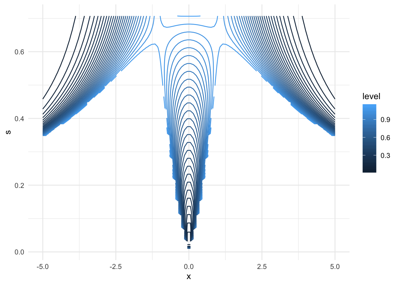
We can see that the function is clearly symmetric in x. Let’s consider then only values of 0 < x < 2.5 and eliminate s < 0.4.
# Update criteria
vals <- vals %>% filter(x > 0, x < 2.5, s > 0.4)
# Plot
ggplot(data = vals, aes(x = x, y = s, z = M)) +
    geom_contour(bins = 100, aes(colour = stat(level)))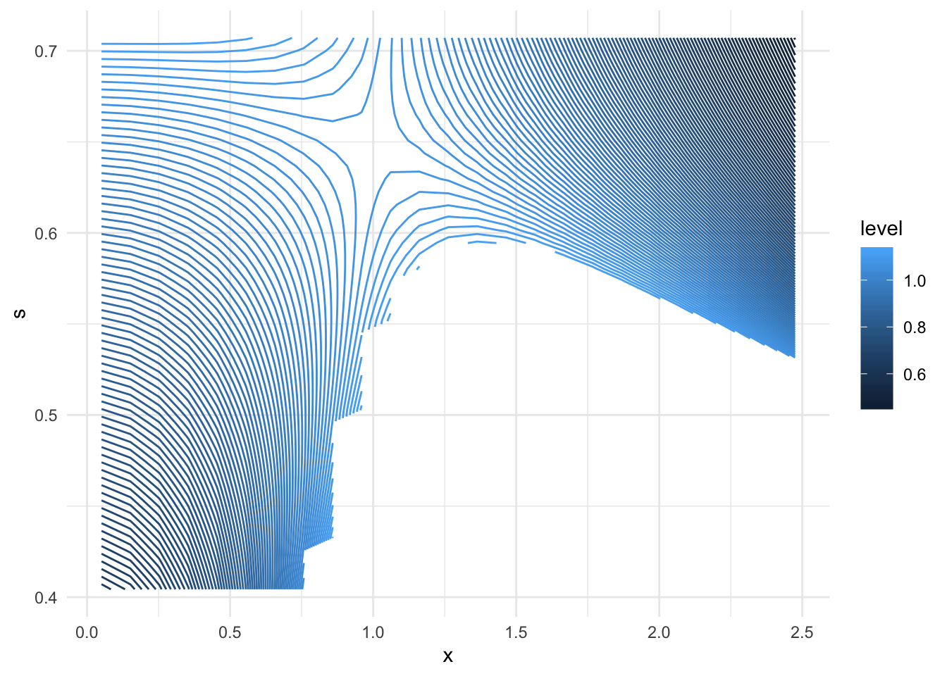
We can see that the optimum is around x = 1 and s ~ 0.65 Let’s narrow down on a square around that:
# Re-generate a denser subsetin that square
s <- seq(from = 0.6, to = 0.7, length.out = 100)
x <- seq(from = 0.5, to = 1.5, length.out = 100)

# Compute the values:
vals <- as.tibble(expand.grid(s,x)) %>% rename(s = Var1, x = Var2)
vals$M <- (dnorm(vals$x)/dlogis(vals$x, location = 0, scale = vals$s))

# Plot:
ggplot(data = vals, aes(x = x, y = s, z = M)) +
    geom_contour(bins = 10, aes(colour = stat(level)))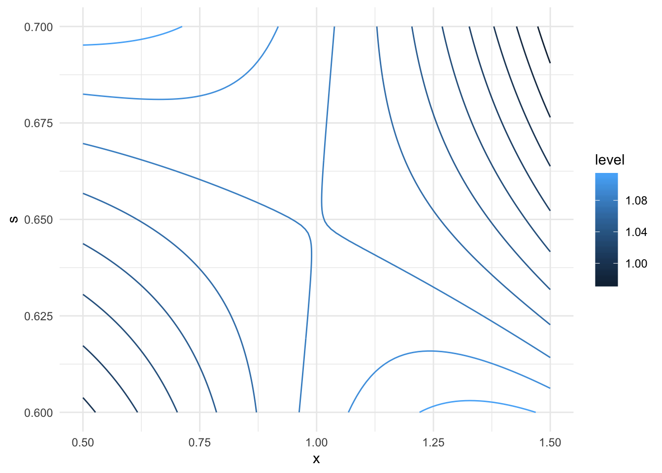
The value at the apparent minimum is M = 1.0808554
#Question 2
##a)
Our goal is to minimize the Loss with respect to \(\theta_j\).
\[\text{Loss}=\sum_{i=1}^n (y_i-\theta_i)^2 + \lambda \sum_{i=2}^{n-1} (\theta_{i+1} -2\theta_i +\theta_{i-1})^2\]
So we begin by differentiating the loss with respect to \(\theta_j\), i.e. taking the gradient. Thankfully a lot of the terms cancel.
\[\frac{d}{d\theta_j} \{(y_j - \theta_j)^2 + (\theta_j - 2\theta_{j-1} + \theta_{j-2})^2 + (\theta_{j+1} - 2\theta_{j} + \theta_{j-1})^2 + (\theta_{j+2} - 2\theta_{j+1} + \theta_{j})^2 \}\]
To find the minimum we have to set the gradient to be 0.
\[0 = \frac{d}{d\theta_j}(\text{Loss})\] \[ 0 = -2(y_j - \theta_j)+ 2\lambda\left( (\theta_j - 2\theta_{j-1} + \theta_{j-2}) -2(\theta_{j+1} - 2\theta_{j} + \theta_{j-1}) + 2(\theta_{j+2} - 2\theta_{j+1} + \theta_{j}) \right) \]
This is where we need to split into cases because of the indexing on the smoothing portion of the loss. To get the \(y_1\) we need to look at index \(i=2\) on the second term in order to get \(\theta_1\). Simplifying the above equations yields the following results:
\[ \begin{array}{rcl} (1+\lambda)\hat{\theta}_1 - 2 \lambda\hat{\theta}_2 + \lambda\hat{\theta}_3 & = y_1 \\ -2\lambda \hat{\theta}_1 + (1+5\lambda)\hat{\theta}_2 - 4\lambda\hat{\theta}_3 + \lambda\hat{\theta}_4 & = y_2\\ \lambda\hat{\theta}_{j-2} -4\lambda\hat{\theta}_{j-1} + (1+6\lambda)\hat{\theta}_j -4\lambda\hat{\theta}_{j+1} + \lambda\hat{\theta}_{j+2} & = y_j & 2 < j <n-1 \\ -2\lambda \hat{\theta}_n + (1+5\lambda)\hat{\theta}_{n-1} - 4\lambda\hat{\theta}_{n-2} + \lambda\hat{\theta}_{n-3} & = y_{n-1} \\ (1+\lambda)\hat{\theta}_n - 2 \lambda\hat{\theta}_{n-1} + \lambda\hat{\theta}_{n-2} & =y_n \end{array}. \]
Which is what we wanted to show.
We can also rewrite the above in matrix notation to get that \(y = A_\lambda \hat{\theta}\) .
##b)
We want to show that if \(y_i\) are linear then \(\hat{\theta}_i = y_i\).
One thing we know is that the Loss function is bounded from below by 0, since it’s a sum of squares.
Then if we plug in \(\hat{\theta}_i = i*a + b\), and noting that the first term is \(0\) for all \(i\):
\[\text{Loss} = \lambda \sum_{i = 2}^{n-1} \left((1+i)a + b - 2ia - 2b +(i-1)a + b \right) = 0\] And since loss is bounded from below by 0 this is the best we can get threfore it is the optimum.
##c)
We notice that A is very sparse (at most 5 non-zero entries per row), but note that \(A = I + B\), where \(I\) is the identity. And \(B\) is such that \(B \theta\) is the second term in the loss Equation. Consider \(C = B^{\frac{1}{2}}\) i.e. A matrix such that:
\[\theta^T C \theta = B\theta\] Since the second term of the loss is strictly non-negative (since it’s the sum of squares), and since all \(\lambda_i > 0\), we know that C is positive definite. We also know that the identity is positive definite. Since C is positive definite we also know that \(C^{2}\) is positive definite but that is just \(B\) so we conclude that A is positive definite. And so the algorithm will converge.
##d)
# This is a template of an R function used to estimate the parameters

seidel <- function(y, lambda, theta, max.iter = 50, eps = 1.e-6) {

    n <- length(y)

    # Define initial estimates if unspecified
    if (missing(theta)) theta <- y

    # Compute objective function for initial estimates
    obj <- sum((y - theta)^2) + lambda * sum(diff(diff(theta))^2)

    # The function diff(diff(theta)) computes second differences of the vector
    # theta
    converged <- FALSE

    # You will need to define convergence (no.conv==F) somehow - either in
    # terms of the objective function or in terms of the estimates
    # Do Gauss-Seidel iteration until convergence or until max.iter iterations
    iter <- 0

    theta_old <- theta

    while (!converged) {
        theta[1] <- (y[1] + 2 * lambda * theta[2] - lambda * theta[3])/(1 + lambda)

        theta[2] <- (y[2] + 2 * lambda * theta[1] +
                        4 * lambda * theta[3] -
                        lambda * theta[4])/(1 + 5*lambda)

        # Update theta[2],..., theta[n-1]
        for (j in 3:(n - 2)) {
            theta[j] <- (y[j] -
                            lambda*theta[j - 2] +
                            4 * lambda * theta[j - 1] +
                            4 * lambda*theta[j + 1] -
                            lambda*theta[j + 2]
                         ) / (1 + 6 * lambda)
        }

        theta[n - 1] <- (y[n - 1] -
                            lambda * theta[n - 3] -
                            4 * lambda * theta[n - 2] +
                            2 * lambda * theta[n]
                         ) / (1 + 5 * lambda)

        theta[n] <- (y[n] -
                        lambda * theta[n - 2] -
                        2 * theta[n - 1]
                     ) / (1 + lambda)

        # Compute new objective function for current estimates
        obj_new <- sum((y - theta)^2) + lambda * sum(diff(diff(theta))^2)

        # Update the iterator
        iter <- iter + 1
        # Now set converged to TRUE if either convergence or iter=max.iter
        # and update the value of the objective function variable obj
        if (abs(obj_new - obj) < eps) converged <- TRUE
        if (iter == max.iter) converged <- TRUE
        obj <- obj_new
        theta_old <- theta
    }

    r <- list(y = y, theta = theta, obj = obj, niters = iter)
    return(r)
}

# take 1000 points to transform into our RV

x <- c(1:1000)/1000

y <- cos(6*pi*x)*exp(-2*x) + rnorm(1000,0,0.05)

# estimates for various smoothing parameters (powers of 5 cause why not)
r0 <- seidel(y,lambda = 0)

r5 <- seidel(y, lambda = 5, theta = r0$theta, max.iter = 1000)

r25 <- seidel(y,lambda = 25, theta = r5$theta, max.iter = 1000)

r125 <- seidel(y,lambda = 125, theta = r25$theta, max.iter = 10000)

# create a tibble for plots
gs_result <- tibble(index = c(1:1000),
                    RV = y,
                    sol0 = r0$theta,
                    sol5 = r5$theta,
                    sol25 = r25$theta,
                    sol125 = r125$theta)

# Plot
g_complete <- ggplot() +
    # plot the real points
    geom_point(data = gs_result,
               aes(x = index, y = RV),
               alpha = 0.4) +
    # plot the first result (no smoothing)
    geom_line(data = gs_result,
              aes(x = index, y = sol0, color = "red"),
              alpha = 0.7) +
    geom_line(data = gs_result,
              aes(x = index, y = sol5, color = "blue"),
              alpha = 0.7) +
    geom_line(data = gs_result,
              aes(x = index, y = sol25, color = "green"),
              alpha = 0.7) +
    geom_line(data = gs_result,
              aes(x = index, y = sol125, color = "black"),
              alpha = 0.7) +
    theme_minimal() +
    labs(title = expression("Estimation of smoothed " ~ theta ~" under various smoothing parameters"),
         x = "Index",
         y = "Random Variable") +
    scale_color_discrete(name = "Y series",
                         labels = c("Lambda = 0 ",
                                    "Lambda = 5",
                                    "Lambda = 25",
                                    "Lambda = 125"))

g_complete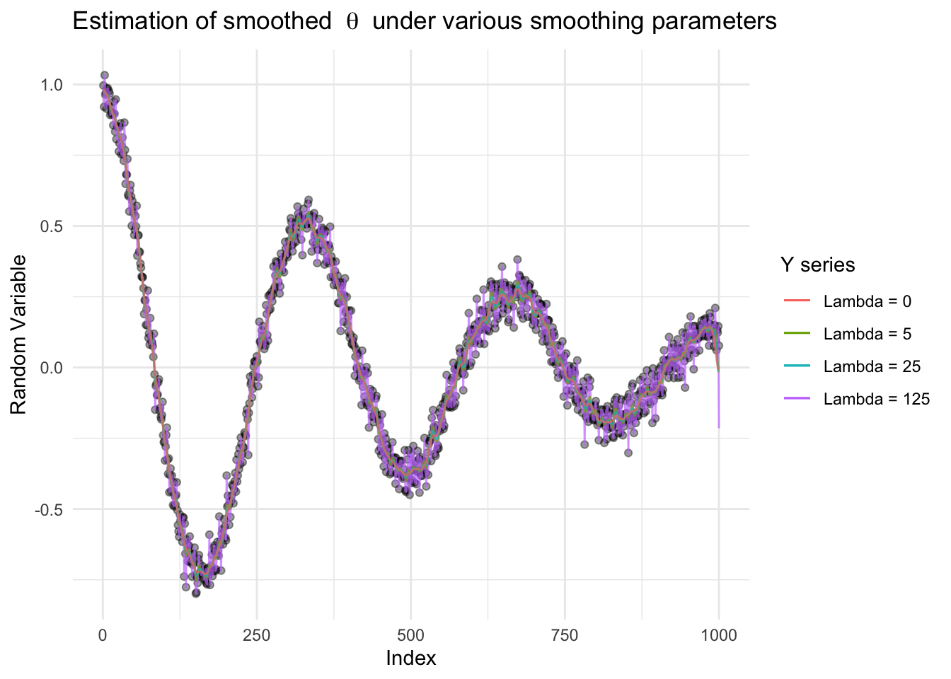
From the graph above we see that as the smoothing parameter lambda increasing, the estimated function becomes smoother (not as many oscillations). This is to say it is not as sensitive to fluctations around the true value.
In particular when zooming between the indices 250 and 350:
# Shorten
gs_result <- gs_result %>% filter(index > 249, index < 351)

# Plot
g_short <- ggplot() +
    # plot the real points
    geom_point(data = gs_result,
               aes(x = index, y = RV),
               alpha = 0.4) +
    # plot the first result (no smoothing)
    geom_line(data = gs_result,
              aes(x = index, y = sol0, color = "red"),
              alpha = 0.7) +
    geom_line(data = gs_result,
              aes(x = index, y = sol5, color = "blue"),
              alpha = 0.7) +
    geom_line(data = gs_result,
              aes(x = index, y = sol25, color = "green"),
              alpha = 0.7) +
    geom_line(data = gs_result,
              aes(x = index, y = sol125, color = "black"),
              alpha = 0.7) +
    theme_minimal() +
    labs(title = expression("Estimation of smoothed " ~ theta ~" under various smoothing parameters"),
         x = "Index",
         y = "Random Variable") +
    scale_color_discrete(name = "Y series",
                         labels = c("Lambda = 0 ",
                                    "Lambda = 5",
                                    "Lambda = 25",
                                    "Lambda = 125"))

g_short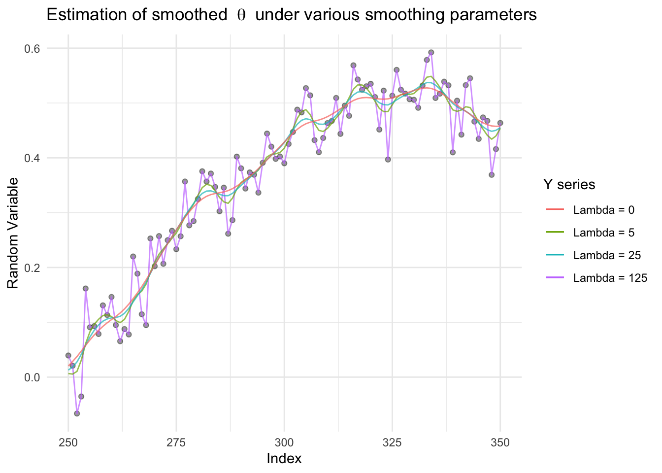
There is not very much difference between lambdas above 5. It could be interesting to look over a grid of lambdas between 0 and 5.