Assignment 1
Michal Malyska
Handout
You can see the handout for this Assignment here
The function fwht2d is provided by prof Knight here
The boats image is also provided in the Assignment here
Setup
set.seed(2718)
knitr::opts_chunk$set(cache = TRUE)
# Libraries
library(tidyverse)

# Function:
source("./STA410_A1_source/fwht2d.txt")

# Data
boats <- matrix(scan("./STA410_A1_source/boats.txt"), ncol = 256, byrow = TRUE)
Question 1
##a) We have:
\[ \hat{Z} = H_mZH_n \]
And we know that:
\[ H_mH_m^T = mI_m \]
and
\[ H_m = H_m^T \]
Want to show:
\[ Z = \frac{H_m\hat{Z}H_n}{mn} \]
It’s easy to see that:
\[ H_m\hat{Z}H_n = H_mH_mZH_nH_n = mI_mZI_nn= mnZ \] Then all that is left is dividing by mn and we are done.
b)
threshold <- function(thresholding_type, data, threshold){
    # Check inputs
    if (!thresholding_type %in% c("soft", "hard")) stop("Thresholding must either be soft or hard")
    # Check data type
    if (class(data) != "matrix") stop("data must be a matrix type")
    # soft thresholding
    if (thresholding_type == "soft") {
        # apply the fwht2d
        xhat <- fwht2d(data)
        # do soft thresholding
        xhat_thr <- sign(xhat)*(pmax(abs(xhat) - threshold, 0))
        # get back to x
        x <- fwht2d(xhat_thr) / length(data)
        # return
        return(x)
    }
    # hard thresholding
    else {
        # apply the fwht2d
        xhat <- fwht2d(data)
        # do hard thresholding
        xhat_thr <- ifelse(test = abs(xhat) > threshold, yes = xhat, no = 0)
        # get back to x
        x <- fwht2d(xhat_thr) / length(data)
        return(x)
    }
}
c)
# to fix some plot issues:
#my_plot_hook <- function(x, options)
#  paste("\n", knitr::hook_plot_tex(x, options), "\n")
#knitr::knit_hooks$set(plot = my_plot_hook)

# original image:
image(boats, axes = FALSE, col = grey(seq(0, 1, length = 256)))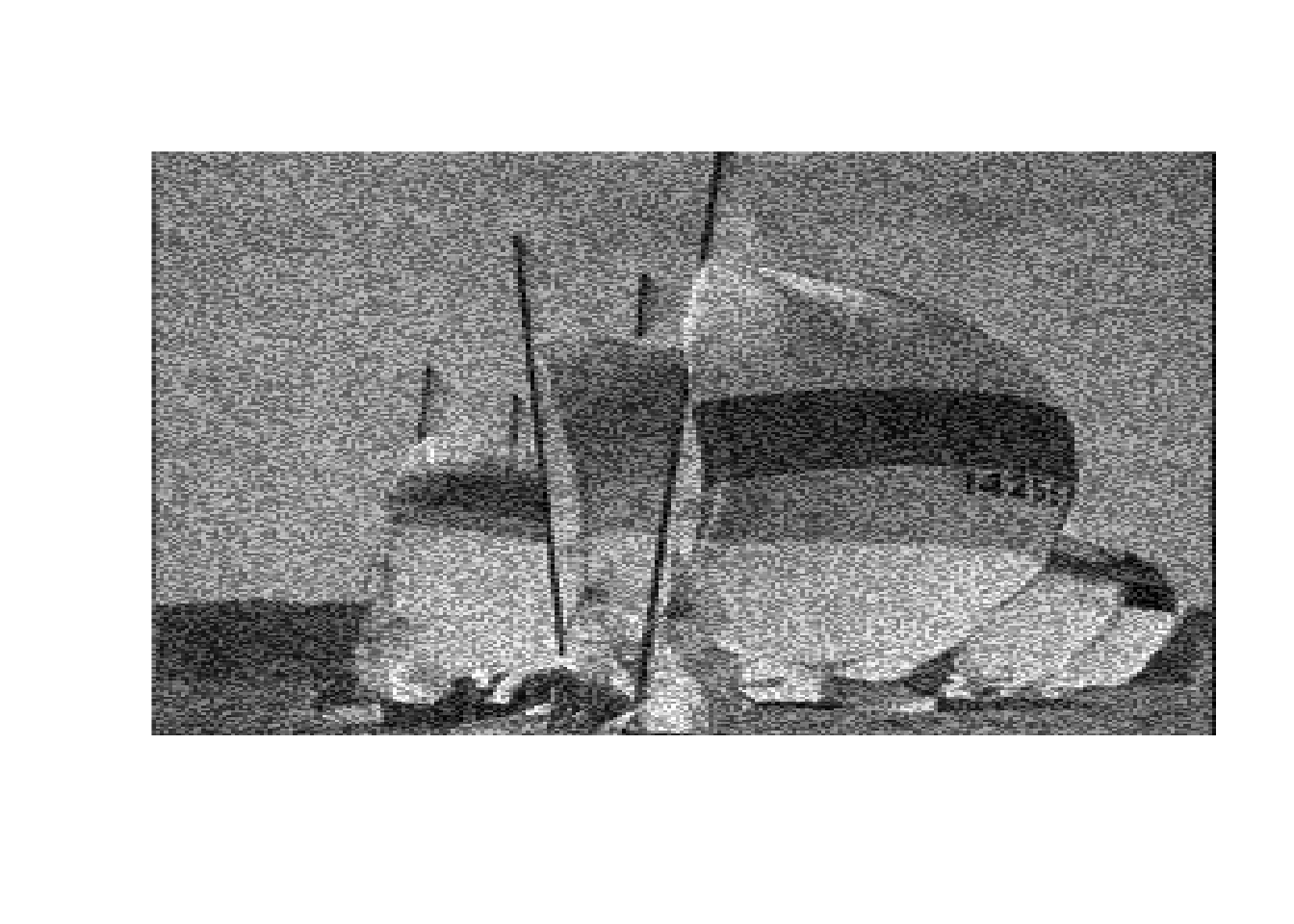
lambdas <- c(1, 2.5, 5, 7.5, 10, 25, 50, 75, 100, 250, 500, 1000)
boats_hard <- threshold("hard", boats, 1)
image(boats_hard, axes = FALSE, col = grey(seq(0, 1, length = 256)))
# plot all thresholded images:
for (lambda in lambdas) {
    boats_hard <- threshold("hard", boats, lambda)
    image(boats_hard, axes = FALSE, col = grey(seq(0, 1, length = 256)),
          main = paste0("Denoised with hard threshold with lambda =", lambda))
    boats_soft <- threshold("soft", boats, lambda)
    image(boats_soft, axes = FALSE, col = grey(seq(0, 1, length = 256)),
          main = paste0("Denoised with soft threshold with lambda =", lambda))
}


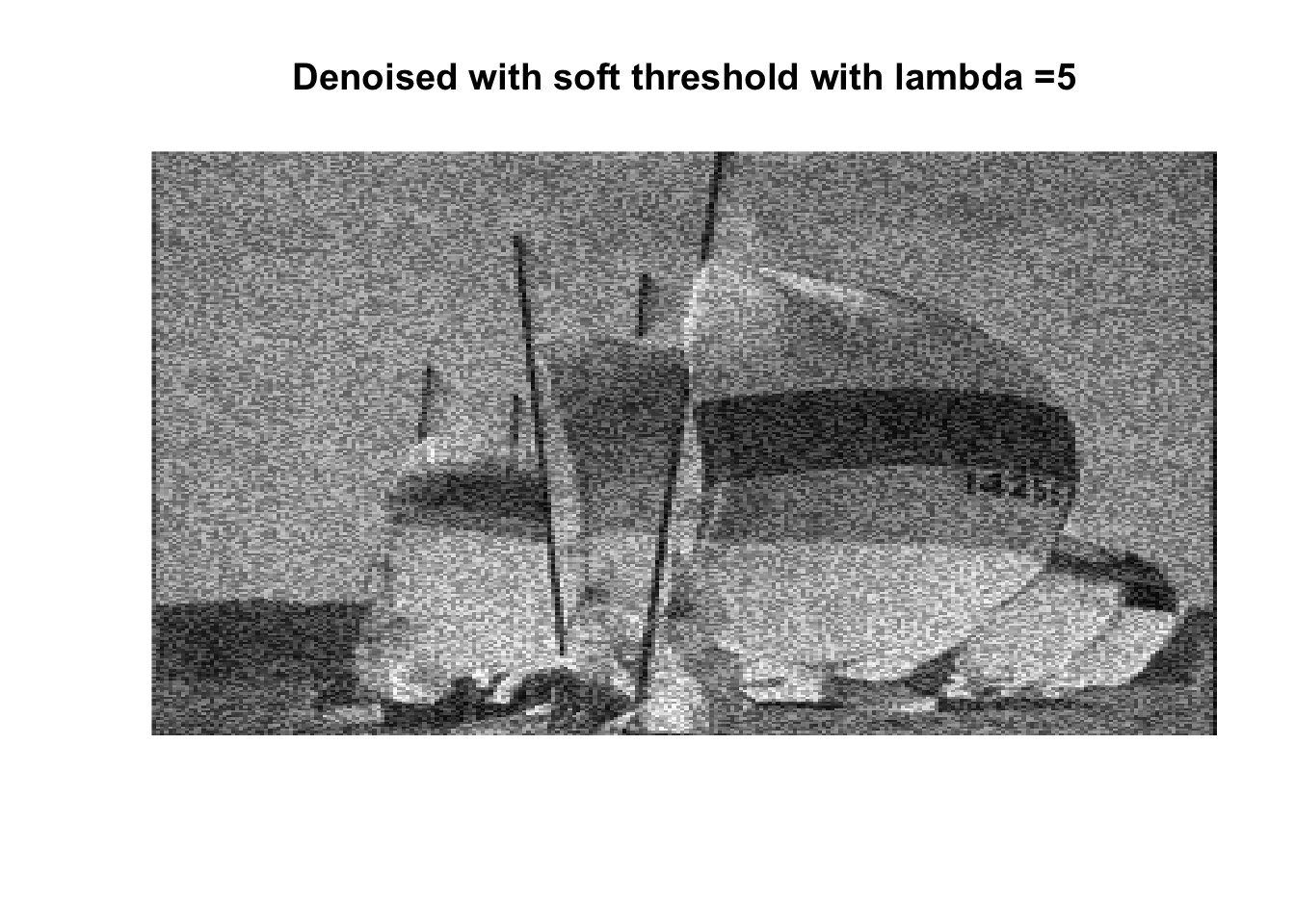
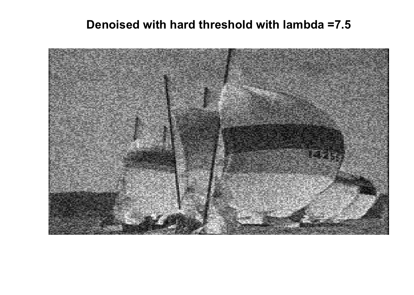


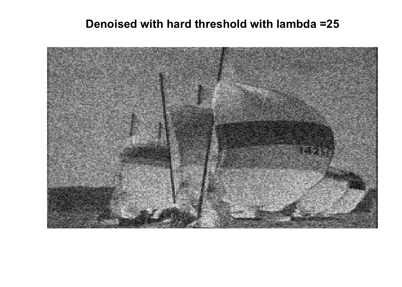


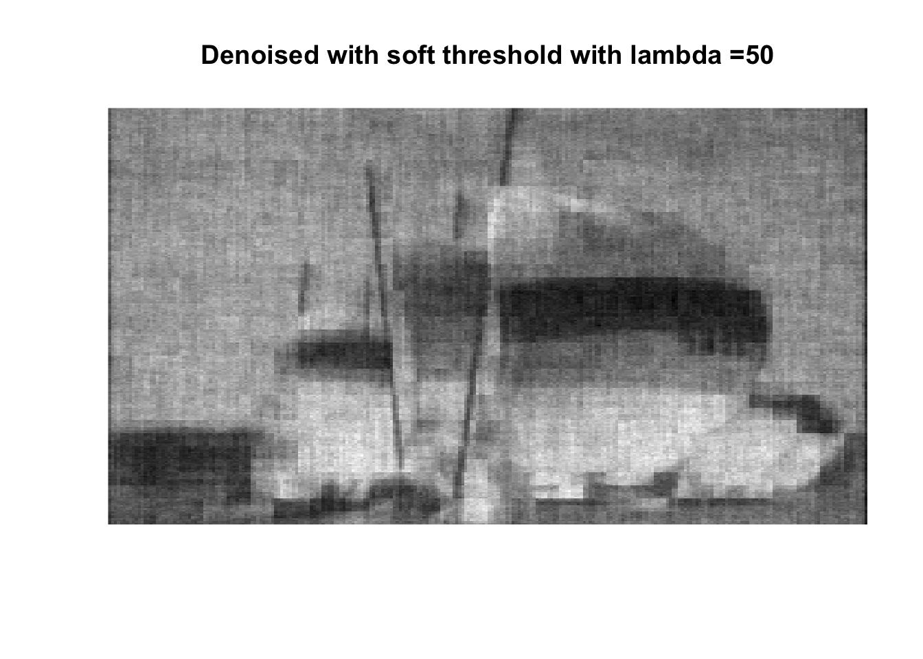


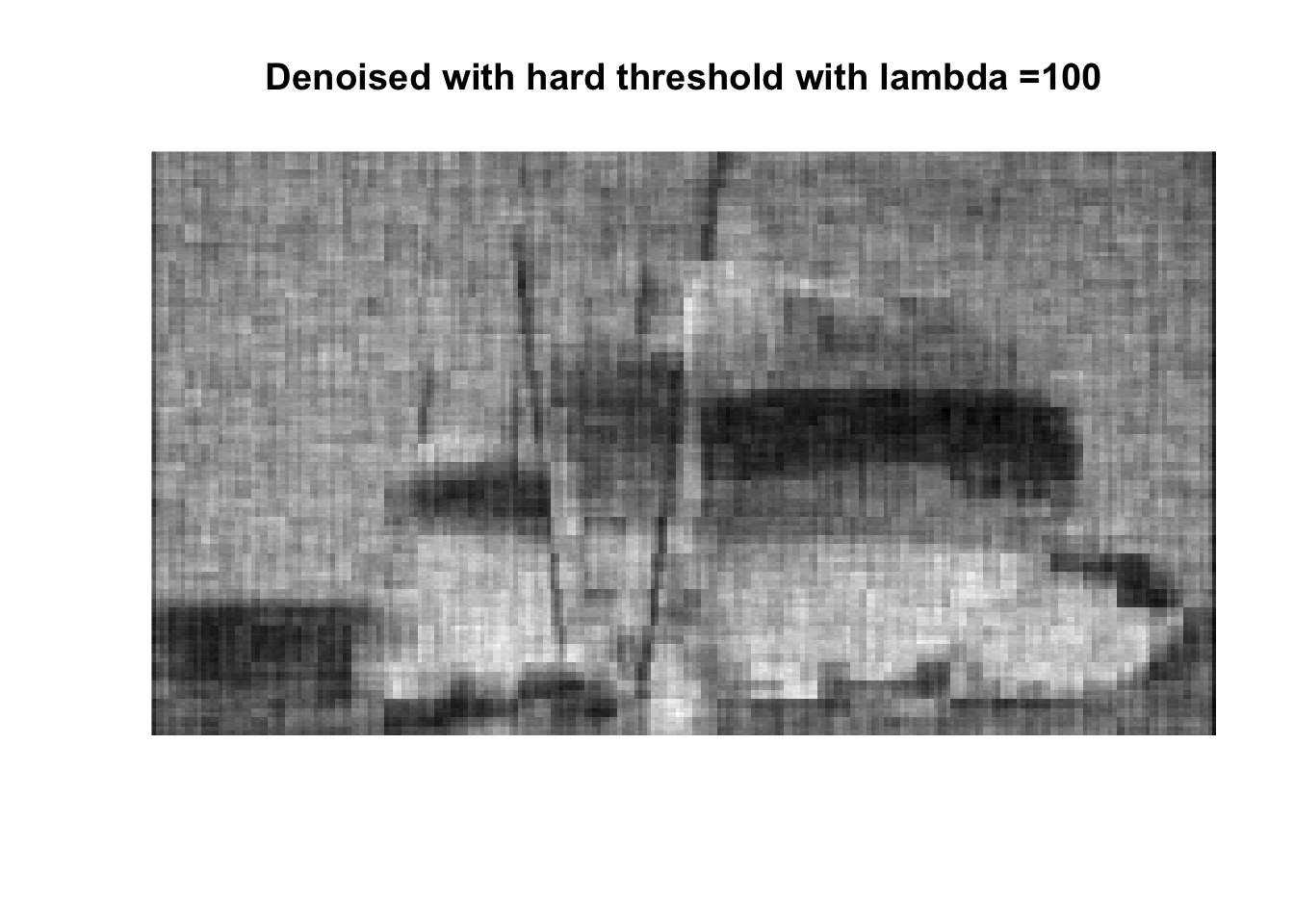
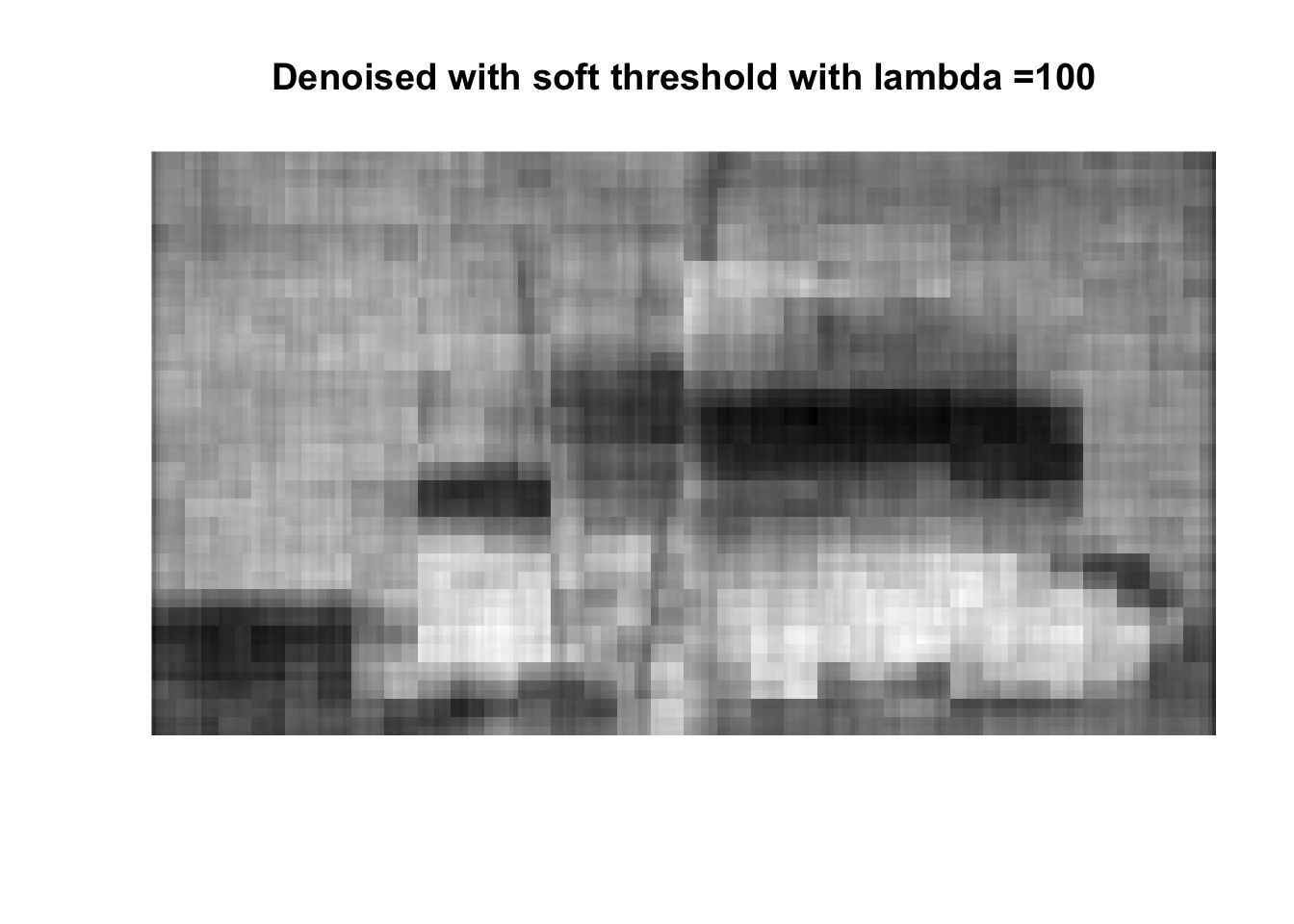
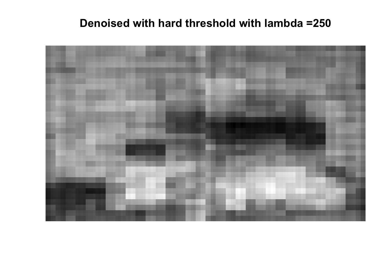

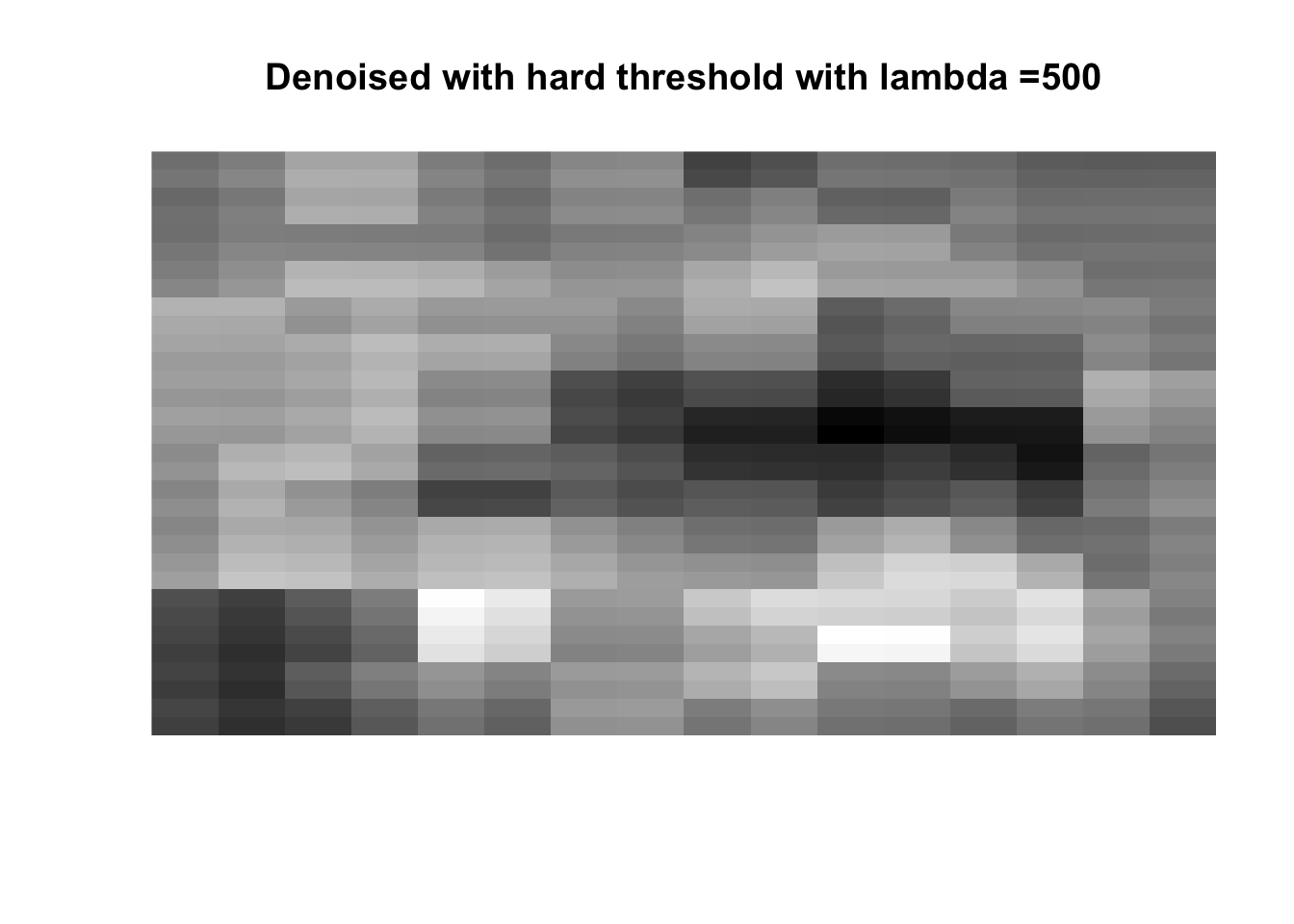
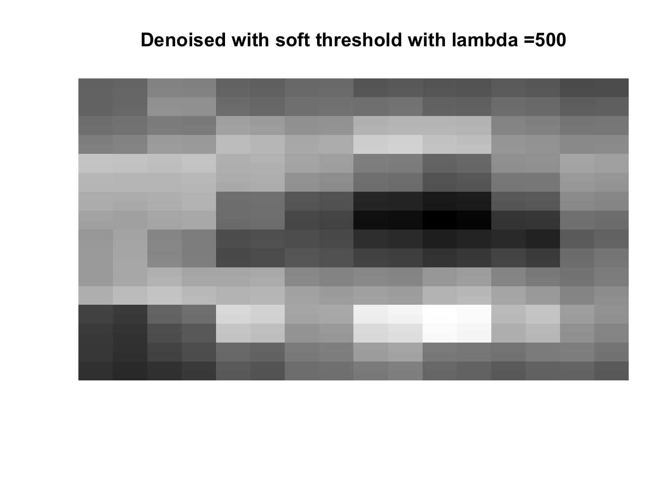
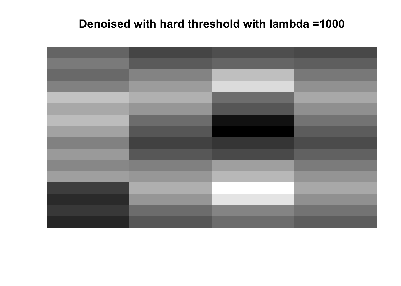
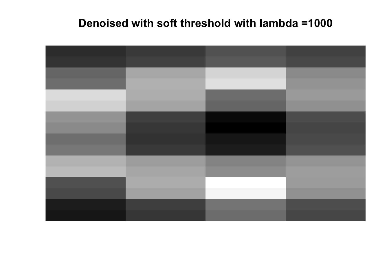
So if you don’t like boats pick 1000, if you like whatever details can exist in a 256x256 pix image, pick 0, otherwise pick 25 with soft thresholding, maybe 50.
Question 2
a) We have:
\[ X_{i} \sim F \] \[ N \sim poiss(\lambda) \] \[ Y = \sum_{i=1}^{N}{X_{i}} ~~ \text{and } ~ N=0 \implies Y=0 \]
and \(N\) and \(X_i\) are independent.
Now take \(\{ X_i \}\) to be discrete, integer valued R.V’s with probability generating function:
\[ \phi(s) = E(s^{X_{i}}) \]
We want to show:
\[ G_Y = g(\phi(s)) = e^{-\lambda(1-\phi(s))} \]
By using independence of X and N we can see the following:
\[ G_Y(s) = E(e^{isY}) = E_N((E(e^{isX}))^N) = E((F(s))^N) = e^{\lambda (\phi(s) -1 )} \]
Which is what we wanted to show.
b)
Show that if \(P(N \geq m) \leq \epsilon\) then \(P(Y \geq ml) \leq \epsilon\) and so we can take \(M \geq ml\).
First note that \(X_i \leq l\) and so \(Y \leq Nl\) Then:
\[ Pr(Y \geq M) \leq Pr(Nl \geq M) = Pr(N \geq \frac{M}{l}) \]
Then just see that :
\[ \exists{m} ~~ s.t. ~~ Pr(N \geq m) \leq \epsilon \implies Pr(Y \geq ml) \leq \epsilon \]
c)
For any given \(s > 1\) i.e. \(s \in S, S = \{ \mathbb{R}^+\setminus (0,1] \}\) we can fix \(M_0\) such that:
\[ \frac{e^{-\lambda(1-\phi(s))}}{s^{M_0}} = \epsilon \] Rearranging we get: \[ M_0 = \frac{-log(\epsilon) - \lambda(1-\phi(s))}{log(s)} \] Then: \[ Pr(Y \geq M_0) \leq \epsilon \] Since this works for any given s, we can take M to be the infimum of all options:
\[ M = M_{min} = \inf_{s \in S} {(\frac{-log(\epsilon) - \lambda(1-\phi(s))}{log(s)})} \]
d)
Computing M:
# Define a function to compute M:

compute_m <- function(lambda, epsilon, px, s){

    # Check condition for c)
    if (!min(s) > 1) {stop("S needs to be greater than 1")}

    # compute the pgf (phi of s in the handout) -----------------------------------

    # initialize
    pgf <- px[1]

    # iterate to get the values:
    for (i in 1:(length(px) - 1)) {
        pgf <- pgf + px[i + 1]*s^i
    }

    # compute M from formula in c) ------------------------------------------------
    all_M <- (-log(epsilon) - lambda*(1 - pgf)) / log(s)
    M <- min(all_M)

    return(list(M, all_M))
}
In our case:
\[ \epsilon = 10^{-5} \]
\[ \lambda = 3 \]
\[ p(x) = P(X_i = x) = \frac{11-x}{66}, ~~ 0 \leq x \leq 10 \]
We need to choose a set of points s such that M is the true infimum. Let’s start with a plot of s from 1.001 to 10 by 0.001 and see the graph of the function we are minimizing.
# define s:
s <- seq(from = 1.001, to = 10, by = 0.001)

# all the other params
epsilon = 10^-5
lambda = 3
px = (11 - c(0:10))/66

# Get the values
M_1 <- compute_m(lambda = lambda, epsilon = epsilon, px = px, s = s)

# Get all M's
ys <- M_1[2][[1]]
# Get the minimum M
M_min <- M_1[1][[1]]

# Store in a tibble
data <- tibble(s = s, y = ys)

# plot
ggplot(data = data, aes(x = s, y = y)) +
    geom_point()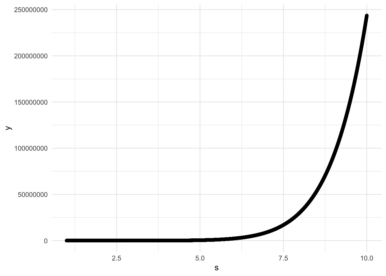
# print for which S is the M minimal
print(data %>% filter(y == M_min))
## # A tibble: 1 x 2
## s y
## <dbl> <dbl>
## 1 1.35 67.2We can clearly see that the function just diverges for large s, and there is a small range where it is highfor values close to 0. Somewhere in between 1 and 2 there is a minimum, so for safety let’s set s to be by 0.0001 between 1.0001 and 2.
s <- seq(from = 1.0001, to = 2, by = 0.0001)
# Get the values
M_1 <- compute_m(lambda = lambda, epsilon = epsilon, px = px, s = s)
# Get all M's
ys <- M_1[2][[1]]
# Get the minimum M:
M_min <- M_1[1][[1]]

# Store in a tibble
data <- tibble(s = s, y = ys)

# plot
ggplot(data = data, aes(x = s, y = y)) +
    geom_point()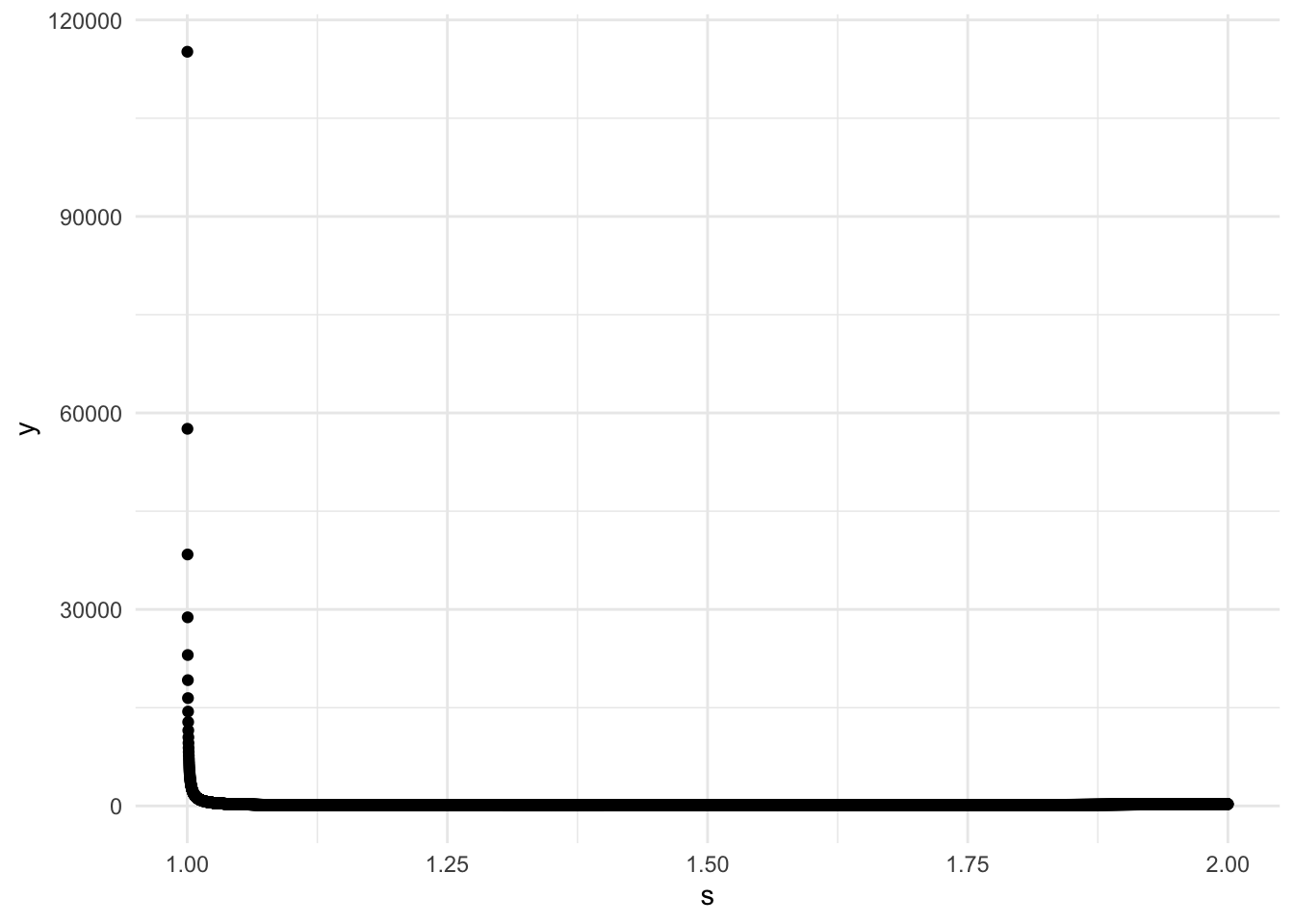
# print for which S is the M minimal
print(data %>% filter(y == M_min))
## # A tibble: 1 x 2
## s y
## <dbl> <dbl>
## 1 1.35 67.2So the optimal M is close to 67, which is a prime, which is horrible. At this point we have a choice of brining M to be the closest power of 2: 128 or just rounding it to \(68 = 2* 2* 17\). I will choose the latter.
Let’s define the compound poisson function:
cpdpoiss <- function(lambda, px, M) {
    # compute for padding
    n <- length(px) - 1
    # pad px with zeros
    px <- c(px, rep(0, M - n - 1))
    # compute the FFT of px
    px_hat <- fft(px)
    # compute py_hat
    py_hat <- exp(-lambda*(1 - px_hat))
    # compute py
    probs <- Re(fft(py_hat, inverse = TRUE))/M

    return(list(y = c(0:(M - 1)), probs = probs))
}
Let’s compute the values we get and plot the result:
# compute
result <- cpdpoiss(lambda, px, 68)
# convert to tibble
result <- tibble(y = result$y, probabilities = result$probs )

# ggplot the result
ggplot(data = result, aes(x = y, y = probabilities)) +
    geom_point() +
    labs(title = "Compound Poisson Distribution") +
    theme_bw() +
    geom_area(fill = "gray", alpha = 0.5)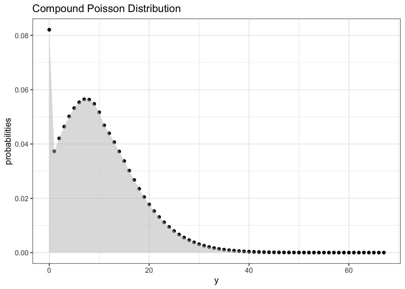
The moral of the story is we could have gotten away with picking \(M = 64\)
Q2 d) Check
For the sake of my sanity I will generate a bunch of observations from this distribution manually to check if it is close to what I have:
# define a function to generate observations

rcpdpoiss <- function(n, lambda, px) {
    # initialize the integers for px
    Xs <- c(0:(length(px) - 1))
    # initialize the results vector
    results <- c(NULL)
    for (i in 1:n) {
        # roll a poisson distribution with mean lambda:
        N <- rpois(n = 1, lambda = lambda)
        # sample N x's and add them up:
        # if result is 0 then set 0
        if (N == 0) {
            Y <- 0
        }
        # otherwise sample N according to px
        else {
            X_i <- sample(x = Xs, size = N, replace = TRUE, prob = px)
            Y = sum(X_i)
        }
        # add to the vector of results
        results <- c(results, Y)
    }
    return(results)
}


# number of observations to generate = 20k
n <- 20000
# Generate the data for our compound poisson
check <- rcpdpoiss(n, lambda, px)
# store in a tibble
emp_data <- tibble(y = check)

# create proportions data
emp_data <- emp_data %>% group_by(y) %>% summarize(count = n()) %>% ungroup()
emp_data$prop <- emp_data$count / n

# Create a comparison between observed and calculated

comparison <- left_join(result, emp_data, by = c("y")) %>% dplyr::select(-count) %>%
    replace_na(list(prop = 0))

ggplot(data = comparison, aes(y)) +
    geom_point(aes(x = y, y = probabilities),color = "red") +
    geom_area(aes(x = y, y = probabilities),fill = "red", alpha = 0.5) +
    geom_point(aes(x = y, y = prop), color = "blue") +
    geom_area(aes(x = y, y = prop), fill = "blue", alpha = 0.5) +
    scale_y_continuous(limits = c(0, 0.1)) +
    ggtitle("Comparison of empirical (blue) vs calculated (red) distribution") +
    theme_bw()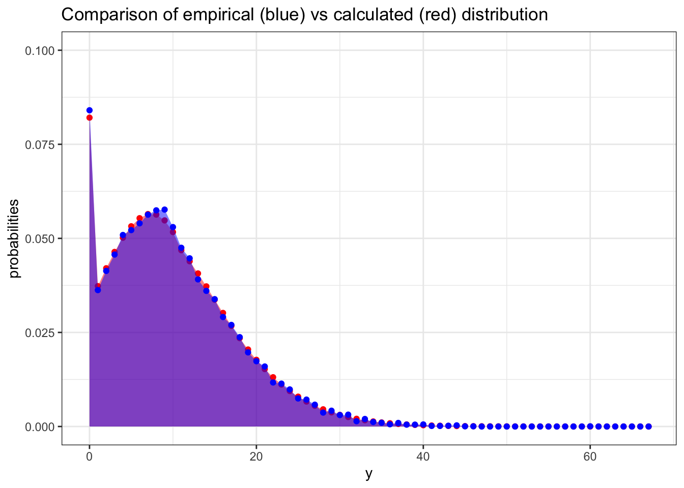
I am very happy with that.