a)

It is very straightforward to see that:

$$\theta_k = \theta_1 + (\theta_2 - \theta_1) + (\theta_3 - \theta_2) + \dots + (\theta_k - \theta_{k-1})$$

$$\text{Since each of the brackets is just } \phi_{j}$$

$$\theta_1 + \sum_{i=2}^{k}\phi_i$$

b)

We compute partial derivative for $g(\theta)$ $$\frac{\partial g(.)}{\partial {\theta_1}} = -2 \sum_{i = 1}^n \left( y_i - \theta_1 + \sum_{j=2}^i \phi_j \right)$$ $$\text{Setting to zero: } \frac{\partial g(.)}{\partial {\theta_1}} = 0$$ $$\text{We obtain: } \theta_1 = \frac{1}{n} \sum_{i = 1}^k \left(y_i-\sum_{j=2}^i\phi_j \right)$$

c)

$$\frac{\partial g(.)}{\partial {\phi_j}} \left( \sum_{i = 1}^n \left(y_i - \theta_1 - \sum_{j=2}^i \phi_j \right)^2 + \lambda \sum_{j = 2}^n | \phi_j | \right) = -2 \sum_{i = j}^n \left(y_i - \theta_1 - \sum_{k=2}^i \phi_k \right) +\lambda \frac{\partial | \phi_j | }{\partial {\phi_j}}$$

Where the $\frac{\partial | \phi_j | }{\partial {\phi_j}}$ will be replaced by a subgradient of the absolute value.

$$\lambda \frac{\partial | \phi_j | }{\partial {\phi_j}} = \begin{cases} \lambda & \phi_j > 0 \\ [- \lambda, \lambda] & \phi_j = 0 \\ - \lambda & \phi_j < 0 \end{cases}$$

Since this is zero only on the set of $[-\lambda, \lambda]$, we know that the overall function is going to be zero only this set as well. Applying that constraint we see:

$$-2 \sum_{i = j}^n \left(y_i - \theta_1 - \sum_{k=2}^i \phi_k \right) \in [-\lambda, \lambda] \\ \iff \\ \left| \sum_{i = j}^n \left(y_i - \theta_1 - \sum_{k=2}^i \phi_k \right) \right| < \frac{\lambda}{2}$$

Now, if $\phi_j \neq 0$ we can see that:

$$\phi_j = \frac{1}{n-j+1} \left( \sum_{i = j}^n \left(y_i - \theta_1 - \sum_{k=2, k \neq j}^i \phi_k \right) - \frac{\lambda}{2} \right) \mbox{for} \sum_{i = j}^n \left(y_i - \theta_1 - \sum_{k=2, k \neq j}^i \phi_k \right) > \frac{\lambda}{2}$$

and the opposite case:

$$\phi_j = \frac{1}{n-j+1} \left( \sum_{i = j}^n \left(y_i - \theta_1 - \sum_{k=2, k \neq j}^i \phi_k \right) + \frac{\lambda}{2} \right) \mbox{for} \sum_{i = j}^n \left(y_i - \theta_1 - \sum_{k=2, k \neq j}^i \phi_k \right) < \frac{\lambda}{2}$$

a)

Let $\theta$ represent the vector of parameters.

First we want to find the loglikelihood: $$\log(L(\theta)) = \sum_{i=1}^n \sum_{k=1}^m u_{ik} \log f_k(x_i) + \sum_{i=1}^n \sum_{k=1}^m u_{ik} \log(\lambda_k)$$

It is only the right sum that depends on the lambda, and solving this problem under the constraint that $\sum_{k=1}^{m}\lambda_k = 1$ It’s easy to see that: $$\hat{\lambda_k} = \frac{1}{n}\sum_{i=1}^n u_{ik}$$

Similarily, plugging in the Normal density for $f_k(.)$ and solving for $\mu$ and $\sigma$ we obtain the other two results:

$$\frac{\partial l(\theta)}{\partial \mu_k} = \frac{1}{\sigma^2_k} \sum_{i=1}^{n}u_{ik}(x_i - \mu_k)$$

$$\frac{\partial l(\theta)}{\partial \sigma^2_k} = - \frac{1}{2 \sigma_k^2} \sum_{i=1}^{n}u_{ik} + \frac{1}{2(\sigma^2_k)^2}\sum_{i=1}^{n}u_{ik}(x_i - \mu_k)^2$$

Setting both to 0 and solving produces:

$$\hat{\mu_k} = \frac{\sum_{i=1}^n u_{ik} x_i}{\sum_{i=1}^n u_{ik}}$$

$$\hat{\sigma_k^2} = \frac{\sum_{i=1}^n u_{ik} (x_i - \hat{\mu}_k)^2}{\sum_{i=1}^n u_{ik}}$$

b) Implement the EM algorithm for the model above.

normalmixture <- function(x,k,mu,sigma,lambda,em.iter=50, eps = 10^-5, debug = FALSE) {
    n <- length(x)
    # Add a tiny perturbation to x
    x <- x + rnorm(length(x), mean = 0, sd = eps)
    x <- sort(x)
    vars <- sigma^2
    means <- mu
    lam <- lambda/sum(lambda)
    delta <- matrix(rep(0,n*k),ncol = k)
    loglik <- NULL
    converged = FALSE
    iter = 0
    while (!converged) {
        loglik_new <- 0
        for (i in 1:n) {
            xi <- x[i]
            for (j in 1:k) {
                mj <- means[j]
                varj <- vars[j]
                denom <- 0
                for (u in 1:k) {
                    mu <- means[u]
                    varu <- vars[u]
                    denom <- denom + lam[u]*dnorm(xi,mu,sqrt(varu))
                }
                delta[i,j] <- lam[j]*dnorm(xi,mj,sqrt(varj))/denom
            }
            loglik_new <- loglik_new + log(denom)  
        }
        for (j in 1:k) {
            deltaj <- as.vector(delta[,j])
            lambda[j] <- mean(deltaj)
            means[j] <- weighted.mean(x = x, w = deltaj)
            vars[j] <- weighted.mean((x - means[j])^2, w = deltaj)
        }
        # Standardize lambdas
        lambda <- lambda / sum(lambda)
        lam <- lambda 
        
        # Iterate again
        iter <- iter + 1
        
        # Print iterations for debugging
        if (debug) {cat("Iteration: ", iter, "\n", "Log Likelihood: ", loglik_new, "\n")}
        
        # Update the first  log likelihood
        if (is.null(loglik)) {
            if (debug) {print("loglik empty reached")}
            loglik = loglik_new
        }
        
        # Check for convergence
        else if (abs(tail(loglik, n = 1) - loglik_new) < eps) {
            if (debug) {print("convergence reached")}
            converged <- TRUE
        }
        
        # Check for num interations
        if (iter == em.iter) {
            print("Number of iterations reached")
            converged <- TRUE}
        
        # If likelihood is infinite then print the params
        if (is.infinite(loglik_new)) {
            cat("Infinite Likelihood", "\n")
            r <- list(mu = means,
              var = vars,
              delta = delta,
              lambda = lambda,
              loglik = loglik,
              iterations = iter)
            return(r)
        }
        
        # Update the log likelihood
        loglik <- c(loglik, loglik_new)
    }
    # return
    r <- list(mu = means,
              var = vars,
              delta = delta,
              lambda = lambda,
              loglik = loglik,
              iterations = iter)
    return(r)
}

c)

df <- tibble(x = buffalo)

df %>% ggplot(aes(x = x, ..density..)) +
    geom_density(bw = 5, fill = "red", alpha = 0.3) +
    labs(title = "Density plot")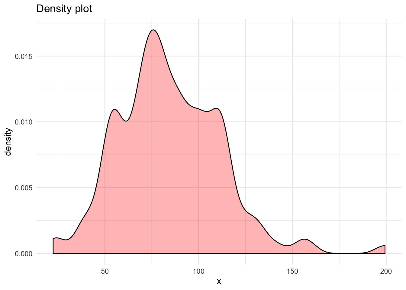

# From density plot:
breaks2 <- c(95)
breaks3 <- c(65, 105)

# Split into normals:
df <- df %>% mutate(bin2 = if_else(x < breaks2[1], 1, 2),
                    bin3 = if_else(x < breaks3[1], 1,
                                   if_else(x < breaks3[2], 2, 3)))

# Calculate the means and variances of each component normals:
norms2 <- df %>% group_by(bin2) %>% summarize(mu = mean(x),
                                              sd = sqrt(var(x)),
                                              count = n())

norms3 <- df %>% group_by(bin3) %>% summarize(mu = mean(x),
                                              sd = sqrt(var(x)),
                                              count = n())


# run this on m = 2
mu_start <- as.vector(norms2$mu)
var_start <- as.vector(norms2$sd)
lambda_start <- as.vector(norms2$count) / length(df$x)

density2 <- normalmixture(df$x, 2, mu_start, var_start, lambda_start, em.iter = 1000, debug = FALSE)

# run this on m = 3 
mu_start <- as.vector(norms3$mu)
var_start <- as.vector(norms3$sd)
lambda_start <- as.vector(norms3$count) / length(df$x)

density3 <- normalmixture(df$x, 3, mu_start, var_start, lambda_start, em.iter = 1000, debug = FALSE)

# Create comparison plot against standard density estimate
density1 <- density(df$x)

## new data: 
df2 <- tibble( x = seq(from = min(df$x), to = max(df$x), length.out = 10000))
df2$density2 <- density2$lambda[1] * dnorm(df2$x, mean = density2$mu[1], sd = sqrt(density2$var[1])) +
    density2$lambda[2] * dnorm(df2$x, mean = density2$mu[2], sd = sqrt(density2$var[2]))
df2$density3 <- density3$lambda[1] * dnorm(df2$x, mean = density3$mu[1], sd = sqrt(density3$var[1])) +
    density3$lambda[2] * dnorm(df2$x, mean = density3$mu[2], sd = sqrt(density3$var[2])) +
    density3$lambda[3] * dnorm(df2$x, mean = density3$mu[3], sd = sqrt(density3$var[3]))

# Make the plot:
ggplot(data = df2, aes(x = df2$x)) +
    geom_point(aes(y = df2$density2), color = "red") +
    geom_point(aes(y = df2$density3), color = "blue") +
    geom_density(data = df, mapping = aes(x = x), fill = "green", alpha = 0.5) +
    labs(main = "Density Estimates at m = 2 (red) and m = 3 (blue)")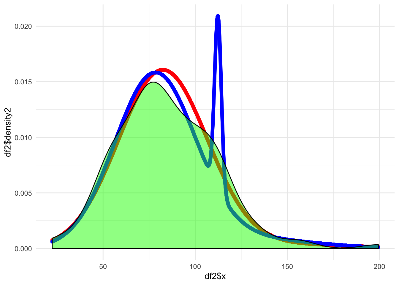

This tiny “hand” looks weird so I will do a sanity check with the mixtools package to see if my work seems reasonable.

mu_start <- as.vector(norms2$mu)
var_start <- as.vector(norms2$sd)
lambda_start <- as.vector(norms2$count) / length(df$x)

density4 <- mixtools::normalmixEM(df$x, k = 2,
                                  mu = mu_start,
                                  sigma = var_start,
                                  lambda = lambda_start)

## number of iterations= 431

mu_start <- as.vector(norms3$mu)
var_start <- as.vector(norms3$sd)
lambda_start <- as.vector(norms3$count) / length(df$x)

density5 <- mixtools::normalmixEM(df$x, k = 3,
                                  mu = mu_start,
                                  sigma = var_start,
                                  lambda = lambda_start)

## number of iterations= 609

print("Mixture of two parameter comparison (mine vs mixtools)")

## [1] "Mixture of two parameter comparison (mine vs mixtools)"

cat("Mean \n",
    density2$mu, "\n",
    density4$mu, "\n")

## Mean 
##  82.33512 150.314 
##  82.41374 153.7458

cat("Variance \n",
    density2$var, "\n",
    density4$sigma^2, "\n")

## Variance 
##  581.1774 1173.335 
##  583.5366 1079.92

cat("Lambda \n",
    density2$lambda, "\n",
    density4$lambda, "\n")

## Lambda 
##  0.9681888 0.03181124 
##  0.970787 0.02921304

print("Mixture of three parameter comparison (mine vs mixtools)")

## [1] "Mixture of three parameter comparison (mine vs mixtools)"

cat("Mean \n",
    density3$mu, "\n",
    density5$mu, "\n")

## Mean 
##  77.98207 112.3513 120.9678 
##  78.01955 112.3522 121.6513

cat("Variance \n",
    density3$var, "\n",
    density5$sigma^2, "\n")

## Variance 
##  471.8441 3.386749 1403.283 
##  473.245 3.383962 1396.149

cat("Lambda \n",
    density3$lambda, "\n",
    density5$lambda, "\n")

## Lambda 
##  0.8340415 0.07175839 0.09420006 
##  0.836254 0.0716751 0.09207088

Looks good to me.

d)

Comparison by AIC:

$$AIC = 2k-2loglikelihood$$

for $m = 2$ we have $2$ means, $2$ variances, and $1$ mixing parameter (since the other one is just 1- the first one) for a total of $k = 5$.

for $m = 3$ we get $k = 8$

Then AIC for both models is:

$$AIC_2 = 10 + 2 \cdot 628.5453 = 1267.091$$

$$AIC_3 = 16 + 2 \cdot 624.3508 = 1264.702$$

Since the AIC has pretty much no difference we can say that both are very comparable. However given the shape of the plots I would prefer the mixture of 2 as it seems to be a much more smooth curve. The fit is also significantly faster.