Reaction Time project EDA
Michal Malyska
# Library Load
# library(summarytools) ## There is a problem with summarytools on the current R version
library(xgboost)
library(lubridate)
library(corrplot)
library(gridExtra)
library(lme4)
# tidyverse at the end so that it doesn't get overwritten.
library(tidyverse)

# Set options
options(scipen = 999)
set.seed(271828)
knitr::opts_chunk$set(cache = TRUE)

# Read the data
df <- read_csv("~/Desktop/University/Undergrad/Statistics/STA490/Reaction Time Project/clean_data.csv")

# See the data
head(df)
## # A tibble: 6 x 11
## ID measurement daytype stimulant hunger fatigue time meq sleep shame
## <dbl> <dbl> <dbl> <dbl> <dbl> <dbl> <chr> <dbl> <dbl> <dbl>
## 1 1 1 1 0 4 4 Morn… 45 6 0
## 2 1 2 1 0 4 3 Earl… 45 6 0
## 3 1 3 1 0 4 5 Late… 45 6 0
## 4 1 4 1 0 3 6 Night 45 6 0
## 5 1 5 0 0 4 2 Morn… 45 10 0
## 6 1 6 0 0 4 3 Earl… 45 10 0
## # … with 1 more variable: reaction <dbl>Let’s start with looking at the distribution of all variables that are meaningful (not ID):
# Convert time (character) variable to factors
df$time <- factor(df$time, levels = c("Morning", "Early Afternoon", "Late Afternoon", "Night"))

# Remove the ones with missing reaction time since that's what we care about
df <- df %>% filter(!is.na(reaction))

# Look at distributions:
df %>% select(-ID) %>% summarize_if(is.numeric,.funs = c("mean", "var"), na.rm = TRUE) %>% t()
## [,1]
## measurement_mean 4.463576159
## daytype_mean 0.506622517
## stimulant_mean 0.122377622
## hunger_mean 4.744897959
## fatigue_mean 3.629251701
## meq_mean 45.180272109
## sleep_mean 7.890025253
## shame_mean 0.079470199
## reaction_mean 0.397589404
## measurement_var 5.299333348
## daytype_var 0.250786561
## stimulant_var 0.107778187
## hunger_var 2.060980706
## fatigue_var 2.042963943
## meq_var 88.230189687
## sleep_var 2.093529192
## shame_var 0.073397725
## reaction_var 0.009209944# Check for missing values in columns:
df %>% summarise_all(funs(sum(is.na(.)))) %>% t()## Warning: funs() is soft deprecated as of dplyr 0.8.0
## Please use a list of either functions or lambdas:
##
## # Simple named list:
## list(mean = mean, median = median)
##
## # Auto named with `tibble::lst()`:
## tibble::lst(mean, median)
##
## # Using lambdas
## list(~ mean(., trim = .2), ~ median(., na.rm = TRUE))
## This warning is displayed once per session.## [,1]
## ID 0
## measurement 0
## daytype 0
## stimulant 16
## hunger 8
## fatigue 8
## time 0
## meq 8
## sleep 38
## shame 0
## reaction 0# Print a text summary of the data
## There is a problem with summarytools on the current R version
# df %>% dfSummary()# See the distribution of reaction times (box and whiskers plot)
ggplot(data = df, aes(y = reaction)) +
geom_boxplot() +
scale_x_continuous(labels = NULL)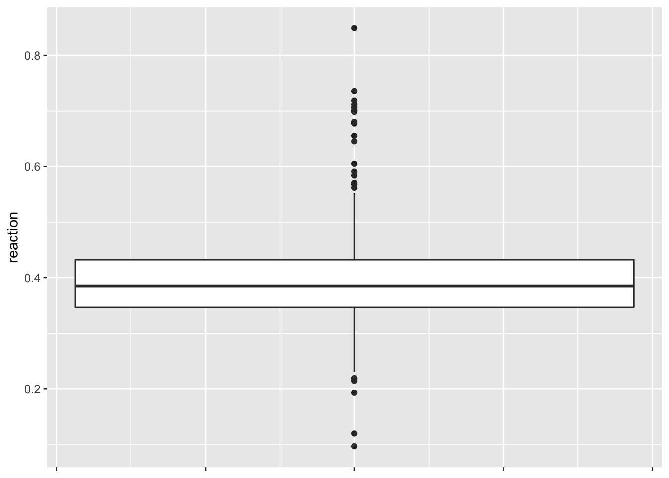
# Since there is a lot of outliers let's look at the histogram and density
ggplot(data = df, aes(x = reaction)) +
    geom_histogram(bins = 30) +
    geom_density(fill = "red", alpha = 0.3)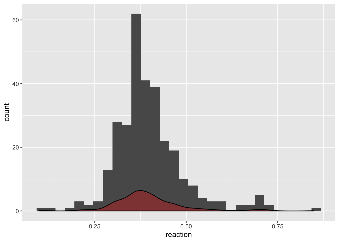
The reaction times seem like a heavy tailed version of a normal distribution. Let’s see if the normal assumption would hold for them:
# QQ plot:
qqnorm(df$reaction)
qqline(df$reaction)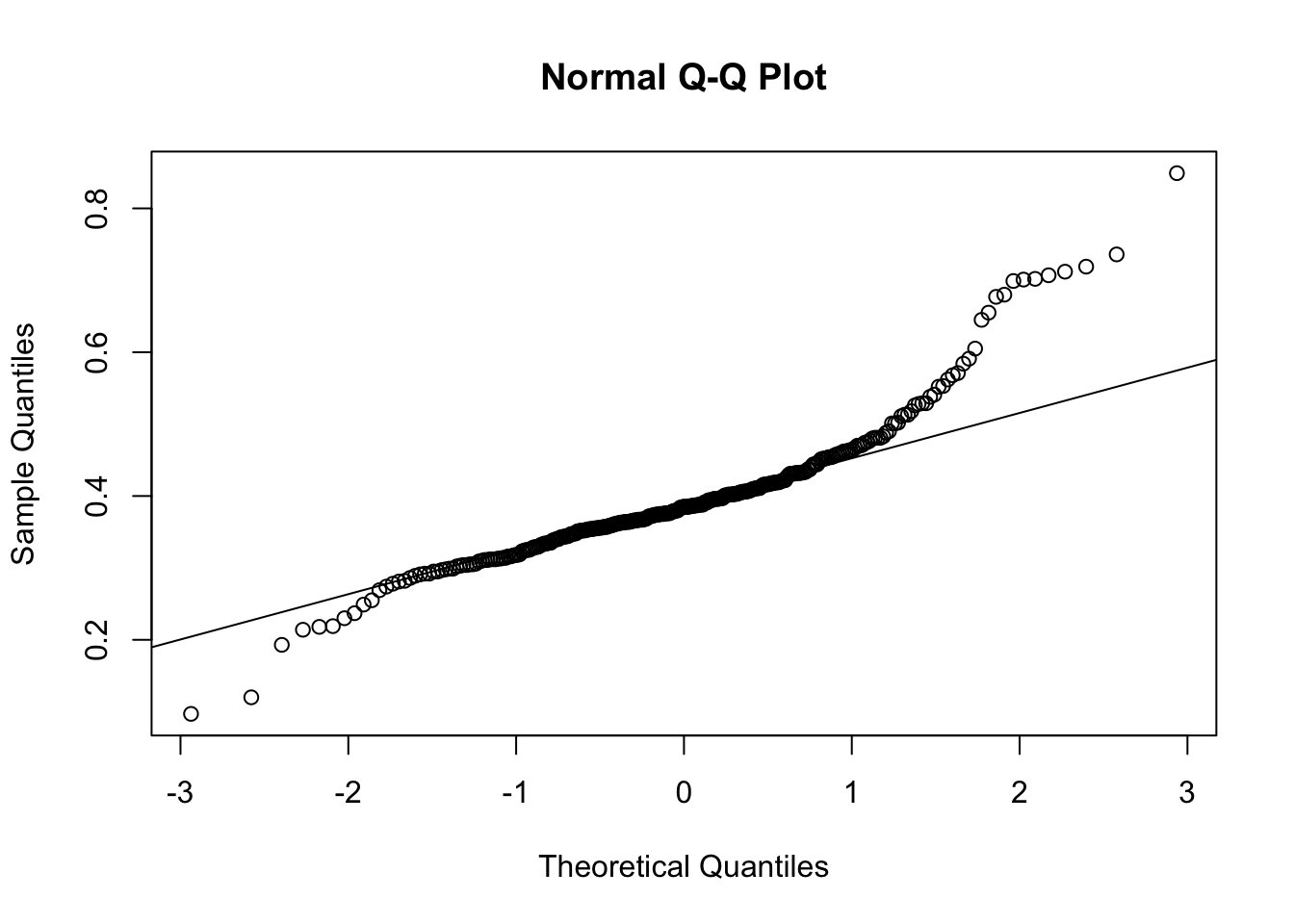
# The heavy tails are clearly visible

# Test of normality:
shapiro.test(df$reaction)
##
## Shapiro-Wilk normality test
##
## data: df$reaction
## W = 0.90255, p-value = 0.0000000000004808So the reaction times are clearly not normally distributed. It does not impact the analysis as of now, but it is good to keep in mind for the future.
The problem statement was to see if the reaction times vary with time of day, let’s see if we have a hint of that in the distribution.
ggplot(data = df, aes(x = time, y = reaction)) +
    geom_point() +
    stat_summary(fun.y = mean,
                 color = "red",
                 geom = "line",
                 aes(group = 1)) + # To plot the line through means of each group
    labs(title = "Reaction Time as a function of circadian rythm time",
         x = "Circadian Time",
         y = "Reaction Time")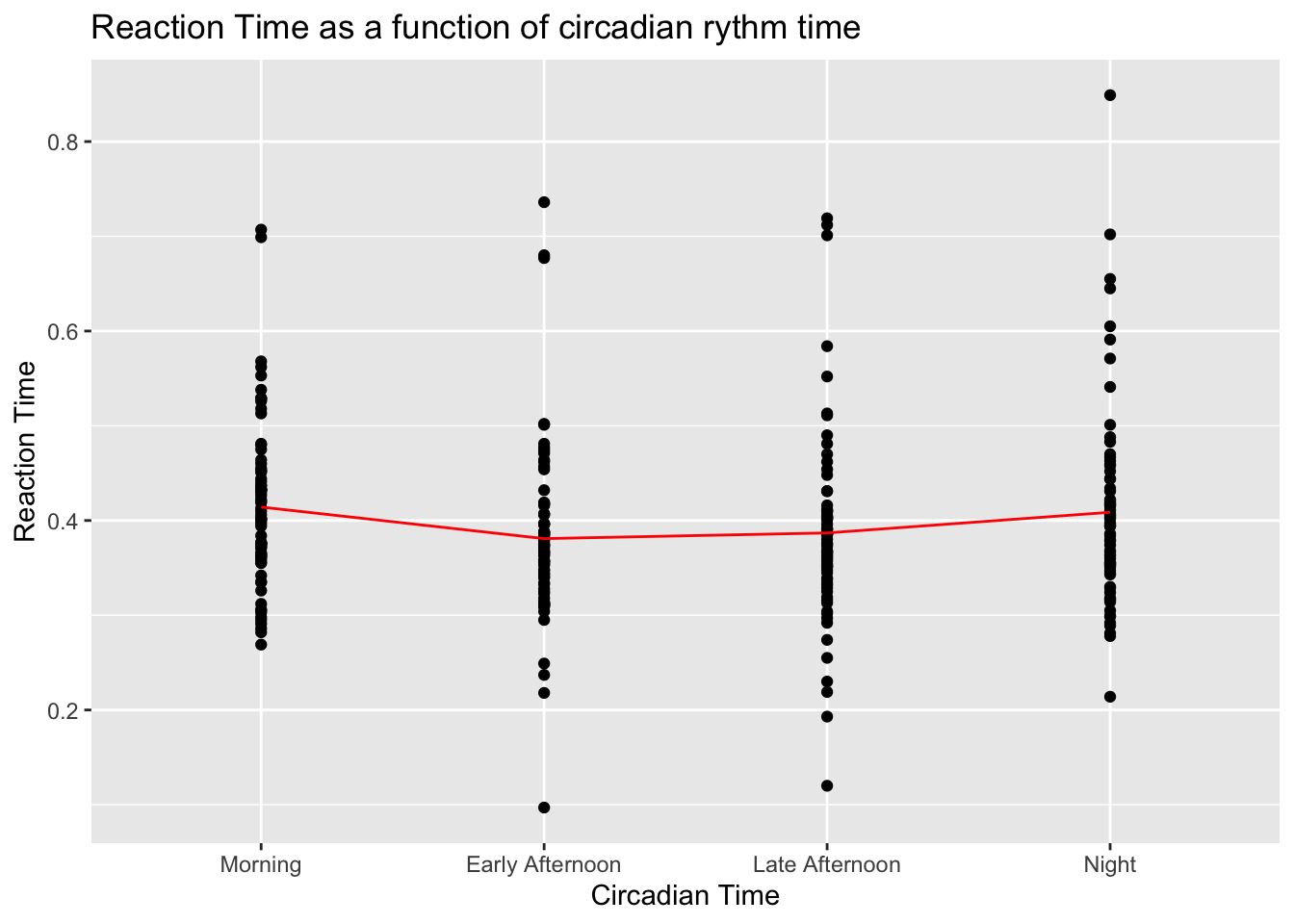
Doesn’t look very promising. Perhaps there is a tiny trend for mornings and nights to be higher, but it’s very hard to tell. There is no point in desting whether means are significantly different since it’s clearly visible with the naked eye that the result will be that they aren’t.
Now let’s see if there are some variables that could explain this better:
# Correlations with reaction times
cor(x = df$reaction, y = df %>% select(-reaction, -ID, -time, -shame) %>% as.matrix,
    use = "complete.obs") %>% t()
## [,1]
## measurement -0.02401558
## daytype 0.06759294
## stimulant -0.03811231
## hunger -0.11937161
## fatigue 0.20047068
## meq -0.16051784
## sleep -0.07622704# Correlation matrix
corrplot(cor(df %>% select(-ID, -reaction, -time, -shame), use = "complete.obs"),
method = "color",
type = "upper",
order = "hclust")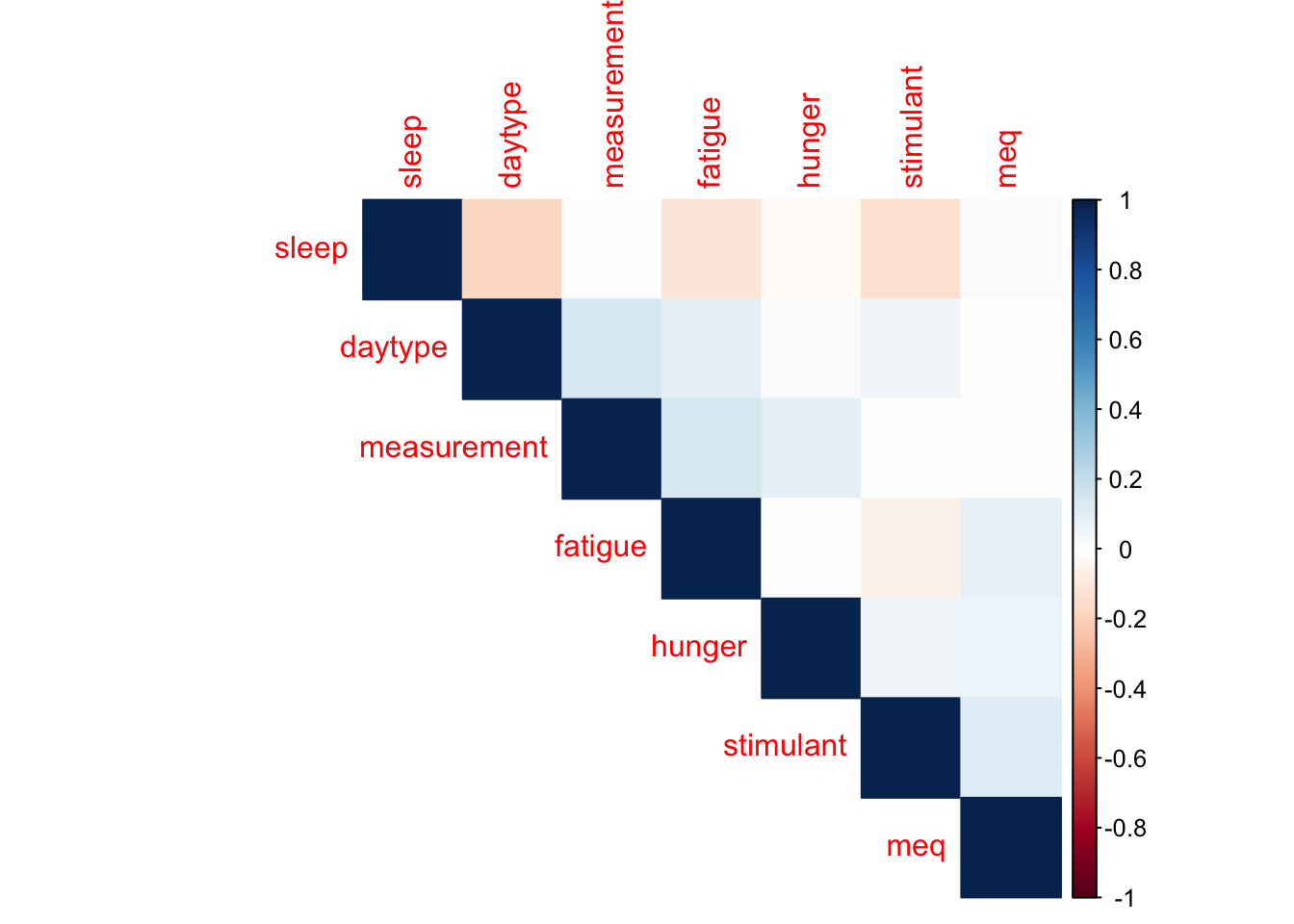
This is very good to see - very low correlations between variables is what we expected, and it means that all our variables have the potential to contribute on their own and have to be considered. We also see very reasonable results: fatigue has the highest correlation with a positive sign (more tired = slower reaction). We also have all the signs that we expect from correlations:
measurement is negatively correlated (so people get better over trials)
daytype is positvely correlated (busier days = slower reaction)
stimulant use is negatively correlated (caffeine = faster reaction)
hunger is negatively correlated (hungry = slower reaction)
sleep is negatively correlated (more sleep = faster reaction)
MEQ will be further investigated as the variable probably needs groupping to be more meaningful.
Let’s see if the time variable could be used at all to predict the reaction times
summary(lm(data = df, formula = reaction ~ time))##
## Call:
## lm(formula = reaction ~ time, data = df)
##
## Residuals:
## Min 1Q Median 3Q Max
## -0.28388 -0.05288 -0.01178 0.02662 0.44030
##
## Coefficients:
## Estimate Std. Error t value Pr(>|t|)
## (Intercept) 0.414208 0.010871 38.102 <0.0000000000000002 ***
## timeEarly Afternoon -0.033325 0.015374 -2.168 0.0310 *
## timeLate Afternoon -0.027341 0.015476 -1.767 0.0783 .
## timeNight -0.005509 0.015583 -0.354 0.7239
## ---
## Signif. codes: 0 '***' 0.001 '**' 0.01 '*' 0.05 '.' 0.1 ' ' 1
##
## Residual standard error: 0.09539 on 298 degrees of freedom
## Multiple R-squared: 0.02178, Adjusted R-squared: 0.01194
## F-statistic: 2.212 on 3 and 298 DF, p-value: 0.08678Short answer: Not really. For the statistically significant indicators, the coefficients are so low that it doesn’t really matter. i.e. the effect size is too small to matter (Very low \(R^2\)) . However there might be some groupping (like adding individual level effects) that could make this predictive.
Now let’s look at the variables on an individual level
# Group by ID
groups <- df %>% group_by(ID)

# Save overall mean and var
reactions_mean <- mean(df$reaction)
reactions_var <- var(df$reaction)

# Plot ID mean reaction times vs overall means

groups %>%
    select(reaction, ID, time) %>%
    group_by(ID, time) %>%
    summarize(mean_reaction_time = mean(reaction)) %>%
    ungroup() %>%
    ggplot(aes(x = time, y = mean_reaction_time)) +
    geom_point() +
    geom_abline(slope = 0, intercept = reactions_mean, color = "red") +
    stat_summary(fun.y = mean, color = "green", geom = "point", size = 3) +
    labs(title = "Individual reaction times vs time",
         caption = "Individual means in black \n time means in green \n overall mean in red")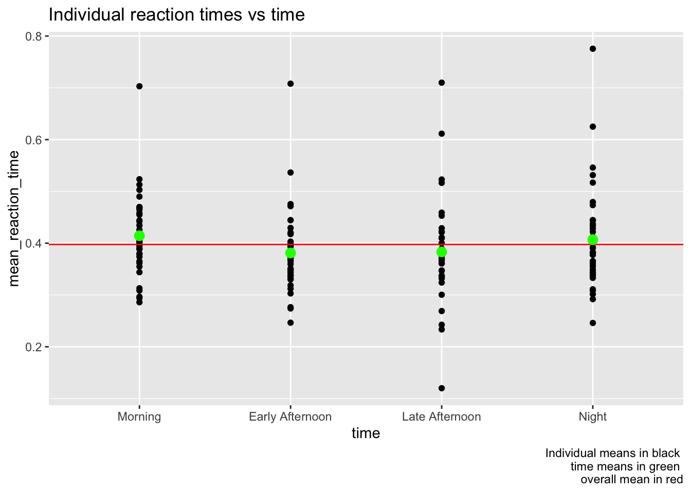
Clearly not much has changed by just groupping by individual. Now let’s try refining the simple linear model fitting a random intercept model based on ID.
mem <- lmer(data = df, formula = reaction ~ time + (1|ID))
summary(mem)
## Linear mixed model fit by REML ['lmerMod']
## Formula: reaction ~ time + (1 | ID)
## Data: df
##
## REML criterion at convergence: -723.7
##
## Scaled residuals:
## Min 1Q Median 3Q Max
## -3.8528 -0.4289 -0.1139 0.4303 4.3735
##
## Random effects:
## Groups Name Variance Std.Dev.
## ID (Intercept) 0.005518 0.07428
## Residual 0.003510 0.05924
## Number of obs: 302, groups: ID, 39
##
## Fixed effects:
## Estimate Std. Error t value
## (Intercept) 0.414306 0.013683 30.280
## timeEarly Afternoon -0.033325 0.009548 -3.490
## timeLate Afternoon -0.028088 0.009620 -2.920
## timeNight -0.006187 0.009699 -0.638
##
## Correlation of Fixed Effects:
## (Intr) tmErlA tmLtAf
## tmErlyAftrn -0.349
## timLtAftrnn -0.346 0.496
## timeNight -0.342 0.492 0.489The model still does not look very good - the variance of residuals is almost as large as the variance of the random effect. The absolute value of t-values reported in the summary also seems very low which implies no statistical significance.
The decision will need to be made whether we consider the variable for day business, as otherwise we will have additional precision at the cost of observations.
Last thing to do is to look over the variable importance as perceived through the eyes of a random forest model. It has the advantage on being able to make decisions based on whether the data is missing (which is the case with this data).
options(na.action = "na.pass")
# Create Model Matrix (one hot encoding)
MM <- model.matrix(df, object = reaction~. -shame -measurement )

# Convert the data to xgboost matrix
dtrain <- xgb.DMatrix(data = MM, label = df$reaction)

# Fit the tree model
xgb_model <- xgboost(data = dtrain,
        max.depth = 5,
        eta = 0.1,
        nrounds = 500,
        booster = "gblinear",
        verbose = 0
        )

# Plot variable importance
var_importance <- xgb.importance(model = xgb_model)

ggplot(var_importance, aes(x = Feature, y = -Weight)) +
    geom_point() +
    theme(axis.text.x = element_text(angle = 45, hjust = 1)) +
    labs(title = "Variable importance")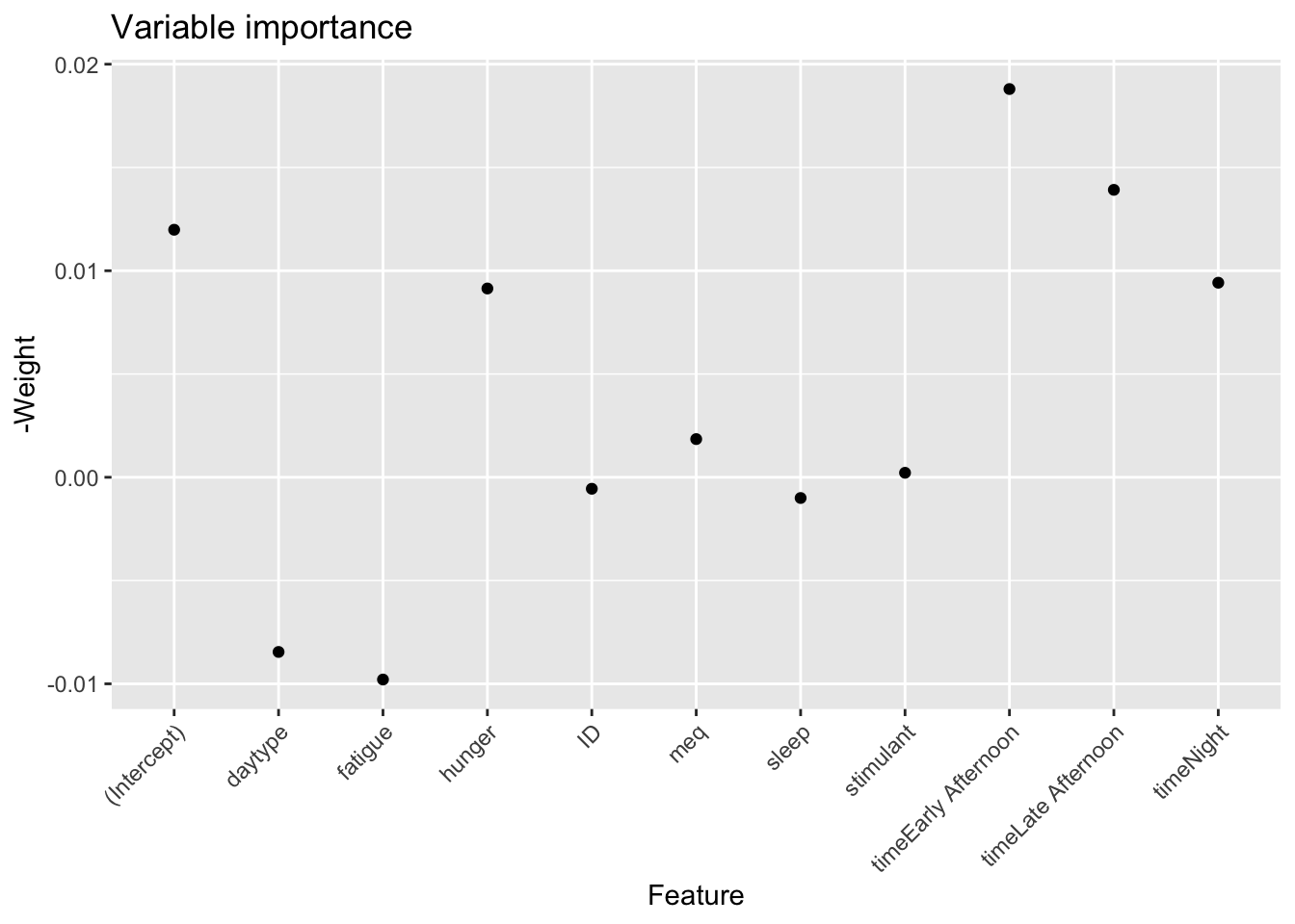
This is a result that shows promise: the most important variables for predicting reaction time are in fact the time of day, and hunger. The Weight is the relative proportion of times the variable was selected to be included in the xgboost component which in our case is a weak linear model.