Preamble

Most of the work in this file is the edited version of solutions provided by Prof. Daniel Simpson who is the instructor for this course.

Source: XKCD

Resources

There is a number of resources available for you to learn and master the tidyverse package. It’s technically not required for the course but it will make your life a lot easier.

Learn R with tidyverse - this on it’s own should give you good enough background to handle most of the coding

Advanced R with tidyverse - most likely far beyond the scope of what’s needed for the course

Cheatsheets - very useful set of cheatsheets

There is a bunch more teaching materials avaialble on Alex’s webiste:

Additional Labs

If you are interested in catching up on some machine learning news, there is a great podcast available - TWIMLAI. If you have some time to spare I highly recommend looking over some of the archival episodes, one of them features a Professor here at UofT Stats - David Duvenaud. It should be very accessible even without a very strong machine learning background. They also have monthly online “meetups” with paper authors discussing stuff in more detail.

Library Load

These are all the libraries we will be using in the course and some additional ones for the extra work done from the R for Data Science textbook:

library(gridExtra)
library(MASS)
library(ISLR)
library(car)
library(modelr)
library(gapminder)
library(broom)
library(ggdendro)
library(dendextend)
library(e1071)
# library(summarytools) ## There is a problem with summarytools on the current R version
library(xgboost)
library(pROC)

# tidyverse goes last so that nothing overwrites the functions
library(tidyverse)
set.seed(217828)
knitr::opts_chunk$set(cache = TRUE)
ggplot2::theme_set(theme_minimal())

Week 1

Week 1 had no tutorials.

Week 2

In the first tutorial we went over the great data notebook by Alex Stringer:

Week 1 Tutorial

Week 3

Question 2

my_kmeans <- function(data, k, n_starts) {
    
done = FALSE # Initialize the condition vector
n = dim(data)[1] #data is a matrix, where each row is one data point

if (k == 1) {
    cluster = rep(1, n) #this vector says which cluster each point is in
    
    centers = apply(
        X = data,
        MARGIN = 2,
        FUN = mean
        ) # Calculate the average distance
    
    cost = sum((data - centers[cluster]) ^ 2) # Compute the cost function for the single cluster
    
    return(list(cluster = cluster, cost = cost)) # Returns a list of [cluster, cost]
}

cluster_old = rep(1, n) # initialize clusters
cost_old = Inf # initialize cost

for (run in 1:n_starts) {
    cluster = rep(1, n) #this vector says which cluster each point is in
    #uniformly choose initial cluster centers
    centers = data[sample(
        x = 1:n,
        size = k,
        replace = FALSE)
    , ] # Sampling datapoints to be cluster centers
    
    while (!done) {
        # Do Step 2.1
        d = matrix(nrow = n, ncol = k) #initialize a matrix of size nxk
        for (j in 1:k) {
            d[, j] = apply(
            X = data,
            MARGIN = 1, #MARGIN = 1 => Rowwise
            FUN = function(d) sum((d - centers[j, ]) ^ 2)
        ) # Computes the cost function for each point for each cluster center
            
        }
        cluster_new = apply(
            X = d,
            MARGIN = 1,
            FUN = which.min
            ) # Take the minimum of the costs
        
# Throw an error if there is a cluster with no points in it
if (length(unique(cluster_new)) < k) stop("Empty cluster!") 

        
# Do Step 2.2
        for (i in 1:k) {
            centers[i, ] = apply(
                X = data[cluster_new == i, ],
                MARGIN = 2, #MARGIN = 2 => Columnwise
                FUN = mean) # Computes mean of the cluster for each cluster
        }
        
# Check if the cluster assignements changed. If they have, set done=TRUE
        if (all(cluster == cluster_new)) {
            done = TRUE
        }
        
        # Update step 
        cluster = cluster_new
    } #end of while not done
    
cost = sum((data - centers[cluster, ]) ^ 2) # Compute the cost

if (cost_old < cost) {
    cluster = cluster_old
    cost = cost_old
    }
    
    cost_old = cost
    cluster_old = cluster
} # if the cost increased, undo

return(list(cluster = cluster, cost = cost))
}

Task : Use this algorithm to make a 4 clustering of the data set in question2.RData. Comment on the clustering.

# Load the data from a data file 
load("~/Desktop/University/Undergrad/Statistics/TA-ing/STA314F18/T2/question2.RData")

# Load the data from a csv file
#data_q2 <- read_csv("Question2_data.csv")


out = my_kmeans(dat_q2 #data 
                , 4 # number of clusters
                , 2 # number of runs
                )

dat_q2$cluster = out$cluster # Assign to the column "cluster" in dat_q2 the column "cluster" in out

dat_q2 %>% ggplot(aes(x = x,y = y)) +
    geom_point(aes(colour = factor(cluster))) #plot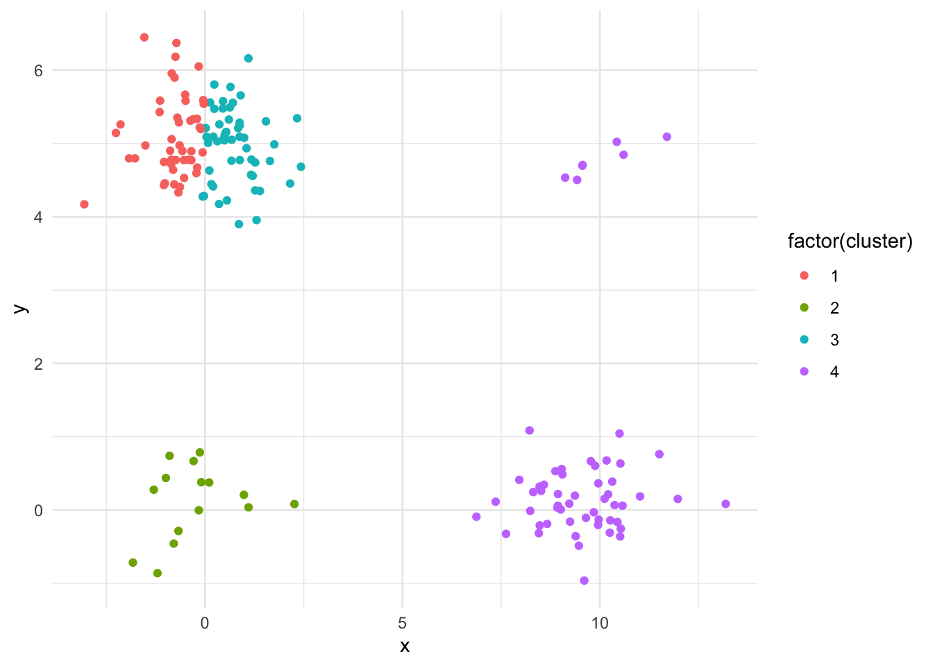

Depending on how many times the kmeans algorithm is run, it sometimes doesn’t find all four distinct clusters. This is due to the uniform intial sampling and the fact that the bottom left and top right clusters are much smaller than the other two. Try increasing the number of runs!

Question 3

# Input the data
d = matrix(c(0, 0.3, 0.4, 0.7,
0.3, 0, 0.5, 0.8,
0.4, 0.5, 0.0, 0.45,
0.7, 0.8, 0.45, 0.0), nrow = 4)


# Set it as distance
d = as.dist(d)

# Plot the clusters with complete linkage:
plot(hclust(d,method = "complete"))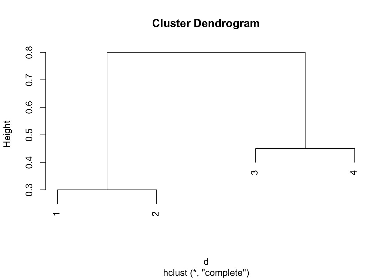

# Plot the clusters with complete linkage:
plot(hclust(d,method = "single"))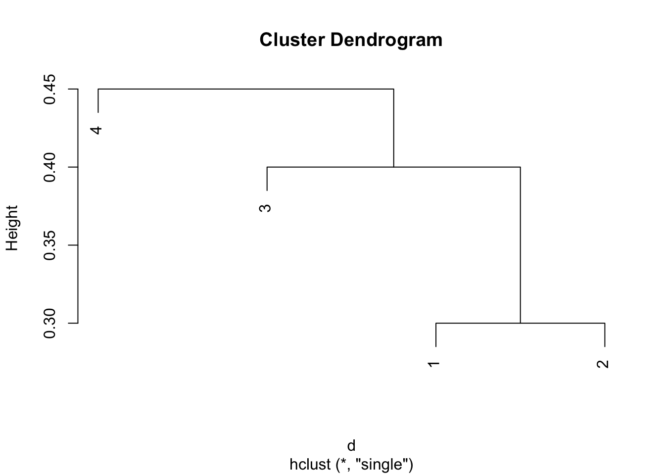

plot(hclust(d,method = "average"))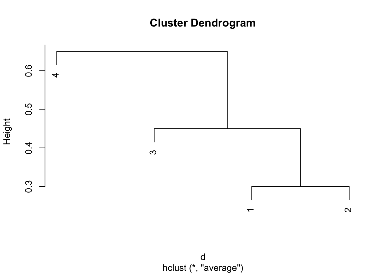

Comparing the two dendrograms, we see that the two clustering from the complete linkage is {1,2}, {3,4}, while the two clustering from the single linkage is {1,2,3}, {4}.

Question 4

For part a) there is not enough information. If the two linkages are equal, then they will fuse at the same hight. Otherwise, the single linkage dendrogram will merge at a lower hight as it only requires one nearby point and not all of the points to be close.

For part b) They’ll merge at the same hight because when you’re just merging single leaves, the linkages all reduce to the distance and are therefore equal.

Week 4

Lab 2

Medium house value (medv) for 506 neighborhoods in Boston. Includes 13 predictors such as: Avg number of rooms in the house, Avg age of houses, socioeconomic status.

# Load the data: (from the MASS package)
data(Boston)

# Check names of variables:
names(Boston)

##  [1] "crim"    "zn"      "indus"   "chas"    "nox"     "rm"      "age"    
##  [8] "dis"     "rad"     "tax"     "ptratio" "black"   "lstat"   "medv"

Let’s try fitting a linear model of medv ~ lstat (socioeconomic status)

# Results in an error - doesn't know where to get the data from.
# lm_fit <- lm(medv ~ lstat)

# Need to specify data = , this is good practice as opposed to following the 
# order set by R inside of the functions most of the time.
lm_fit <- lm(data = Boston, formula = medv ~ lstat)

Now let’s see what the result of the lm function looks like:

# Basic information:
lm_fit

## 
## Call:
## lm(formula = medv ~ lstat, data = Boston)
## 
## Coefficients:
## (Intercept)        lstat  
##       34.55        -0.95

# More comprehensive:
summary(lm_fit)

## 
## Call:
## lm(formula = medv ~ lstat, data = Boston)
## 
## Residuals:
##     Min      1Q  Median      3Q     Max 
## -15.168  -3.990  -1.318   2.034  24.500 
## 
## Coefficients:
##             Estimate Std. Error t value            Pr(>|t|)    
## (Intercept) 34.55384    0.56263   61.41 <0.0000000000000002 ***
## lstat       -0.95005    0.03873  -24.53 <0.0000000000000002 ***
## ---
## Signif. codes:  0 '***' 0.001 '**' 0.01 '*' 0.05 '.' 0.1 ' ' 1
## 
## Residual standard error: 6.216 on 504 degrees of freedom
## Multiple R-squared:  0.5441, Adjusted R-squared:  0.5432 
## F-statistic: 601.6 on 1 and 504 DF,  p-value: < 0.00000000000000022

# What are the contents of lm?
names(lm_fit)

##  [1] "coefficients"  "residuals"     "effects"       "rank"         
##  [5] "fitted.values" "assign"        "qr"            "df.residual"  
##  [9] "xlevels"       "call"          "terms"         "model"

# Extracting p-values:

## Save the summary(lm) as an object! 
sum_lm <- summary(lm_fit)

## P-values are stored with coefficients in the fourth column:
### Intercept P-value:
sum_lm$coefficients[,4][1]

##                                                                                                                                                                                                                                          (Intercept) 
## 0.00000000000000000000000000000000000000000000000000000000000000000000000000000000000000000000000000000000000000000000000000000000000000000000000000000000000000000000000000000000000000000000000000000000000000000000000000000000000000000003743081

### lstat P-value:
sum_lm$coefficients[,4][2]

##                                                                                            lstat 
## 0.0000000000000000000000000000000000000000000000000000000000000000000000000000000000000005081103

# Or you can just call it directly:
summary(lm_fit)$coefficients[,4][1]

##                                                                                                                                                                                                                                          (Intercept) 
## 0.00000000000000000000000000000000000000000000000000000000000000000000000000000000000000000000000000000000000000000000000000000000000000000000000000000000000000000000000000000000000000000000000000000000000000000000000000000000000000000003743081

Now how about predicting and plotting the data:

# Find the intervals for new data

# Confidence intervals:
predict(lm_fit, data.frame(lstat = c(5, 10, 15)),
        interval = 'confidence')

##        fit      lwr      upr
## 1 29.80359 29.00741 30.59978
## 2 25.05335 24.47413 25.63256
## 3 20.30310 19.73159 20.87461

# Prediction interals: 
predict(lm_fit, data.frame(lstat = c(5, 10, 15)),
        interval = 'prediction')

##        fit       lwr      upr
## 1 29.80359 17.565675 42.04151
## 2 25.05335 12.827626 37.27907
## 3 20.30310  8.077742 32.52846

# Plotting:
plot(Boston$lstat, Boston$medv)
abline(lm_fit)

# Playing around with base graphics
plot(Boston$lstat, Boston$medv)
abline(lm_fit ,lwd = 3)
abline(lm_fit ,lwd = 3,col = "red")

plot(Boston$lstat ,Boston$medv ,col = "red")

plot(Boston$lstat ,Boston$medv ,pch = 20)

plot(Boston$lstat ,Boston$medv ,pch = "+")

# Some available symbols:
plot(1:20, 1:20, pch = 1:20)

# Plotting multiple plots on the same line
par(mfrow = c(2,2))

# plot diagnostics
plot(lm_fit)

# revert back to 1 plot per plot
par(mfrow = c(1,1))

plot(predict(lm_fit), residuals(lm_fit))

plot(predict(lm_fit), rstudent(lm_fit)) # standardized residuals

# We observe non-linearity - compute the leverage stats and see which one has the largest
plot(hatvalues(lm_fit))

# Which observation has the highest leverage:
which.max(hatvalues(lm_fit))

## 375 
## 375

# Or plotting using ggplot:
p <- ggplot(data = Boston, aes(x = lstat, y = medv))
p <- p + geom_point()
p <- p + geom_smooth(method = "lm", colour = "red")
p <- p + theme_bw()
p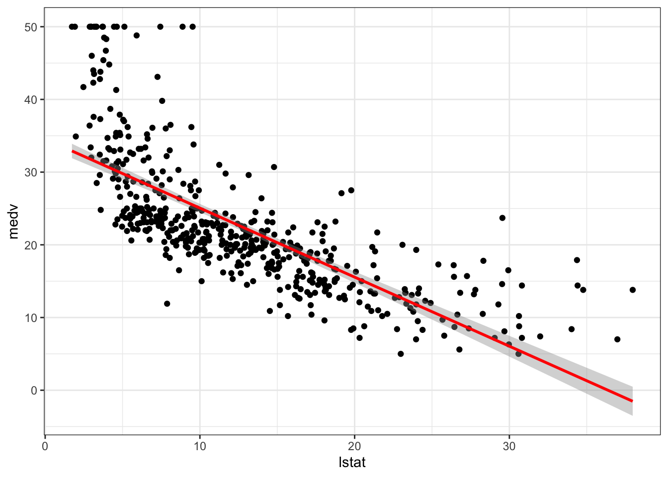

# We can add age to our model (without the interaction)
lm_fit2 <- lm(medv ~ lstat + age, data = Boston)
summary(lm_fit2)

## 
## Call:
## lm(formula = medv ~ lstat + age, data = Boston)
## 
## Residuals:
##     Min      1Q  Median      3Q     Max 
## -15.981  -3.978  -1.283   1.968  23.158 
## 
## Coefficients:
##             Estimate Std. Error t value             Pr(>|t|)    
## (Intercept) 33.22276    0.73085  45.458 < 0.0000000000000002 ***
## lstat       -1.03207    0.04819 -21.416 < 0.0000000000000002 ***
## age          0.03454    0.01223   2.826              0.00491 ** 
## ---
## Signif. codes:  0 '***' 0.001 '**' 0.01 '*' 0.05 '.' 0.1 ' ' 1
## 
## Residual standard error: 6.173 on 503 degrees of freedom
## Multiple R-squared:  0.5513, Adjusted R-squared:  0.5495 
## F-statistic:   309 on 2 and 503 DF,  p-value: < 0.00000000000000022

# We can use all the variables available:
lm_fit3 <- lm(medv ~ ., data = Boston)
summary(lm_fit3)

## 
## Call:
## lm(formula = medv ~ ., data = Boston)
## 
## Residuals:
##     Min      1Q  Median      3Q     Max 
## -15.595  -2.730  -0.518   1.777  26.199 
## 
## Coefficients:
##                Estimate  Std. Error t value             Pr(>|t|)    
## (Intercept)  36.4594884   5.1034588   7.144    0.000000000003283 ***
## crim         -0.1080114   0.0328650  -3.287             0.001087 ** 
## zn            0.0464205   0.0137275   3.382             0.000778 ***
## indus         0.0205586   0.0614957   0.334             0.738288    
## chas          2.6867338   0.8615798   3.118             0.001925 ** 
## nox         -17.7666112   3.8197437  -4.651    0.000004245643808 ***
## rm            3.8098652   0.4179253   9.116 < 0.0000000000000002 ***
## age           0.0006922   0.0132098   0.052             0.958229    
## dis          -1.4755668   0.1994547  -7.398    0.000000000000601 ***
## rad           0.3060495   0.0663464   4.613    0.000005070529023 ***
## tax          -0.0123346   0.0037605  -3.280             0.001112 ** 
## ptratio      -0.9527472   0.1308268  -7.283    0.000000000001309 ***
## black         0.0093117   0.0026860   3.467             0.000573 ***
## lstat        -0.5247584   0.0507153 -10.347 < 0.0000000000000002 ***
## ---
## Signif. codes:  0 '***' 0.001 '**' 0.01 '*' 0.05 '.' 0.1 ' ' 1
## 
## Residual standard error: 4.745 on 492 degrees of freedom
## Multiple R-squared:  0.7406, Adjusted R-squared:  0.7338 
## F-statistic: 108.1 on 13 and 492 DF,  p-value: < 0.00000000000000022

# We can use all the variables but one:
lm_fit4 <- lm(medv ~ . -age, data = Boston)
summary(lm_fit4)

## 
## Call:
## lm(formula = medv ~ . - age, data = Boston)
## 
## Residuals:
##      Min       1Q   Median       3Q      Max 
## -15.6054  -2.7313  -0.5188   1.7601  26.2243 
## 
## Coefficients:
##               Estimate Std. Error t value             Pr(>|t|)    
## (Intercept)  36.436927   5.080119   7.172   0.0000000000027155 ***
## crim         -0.108006   0.032832  -3.290             0.001075 ** 
## zn            0.046334   0.013613   3.404             0.000719 ***
## indus         0.020562   0.061433   0.335             0.737989    
## chas          2.689026   0.859598   3.128             0.001863 ** 
## nox         -17.713540   3.679308  -4.814   0.0000019671100076 ***
## rm            3.814394   0.408480   9.338 < 0.0000000000000002 ***
## dis          -1.478612   0.190611  -7.757   0.0000000000000503 ***
## rad           0.305786   0.066089   4.627   0.0000047505389684 ***
## tax          -0.012329   0.003755  -3.283             0.001099 ** 
## ptratio      -0.952211   0.130294  -7.308   0.0000000000010992 ***
## black         0.009321   0.002678   3.481             0.000544 ***
## lstat        -0.523852   0.047625 -10.999 < 0.0000000000000002 ***
## ---
## Signif. codes:  0 '***' 0.001 '**' 0.01 '*' 0.05 '.' 0.1 ' ' 1
## 
## Residual standard error: 4.74 on 493 degrees of freedom
## Multiple R-squared:  0.7406, Adjusted R-squared:  0.7343 
## F-statistic: 117.3 on 12 and 493 DF,  p-value: < 0.00000000000000022

# Can also update the previous model variables to exclude age:
update(lm_fit3, ~ . -age)

## 
## Call:
## lm(formula = medv ~ crim + zn + indus + chas + nox + rm + dis + 
##     rad + tax + ptratio + black + lstat, data = Boston)
## 
## Coefficients:
## (Intercept)         crim           zn        indus         chas          nox  
##   36.436927    -0.108006     0.046334     0.020562     2.689026   -17.713540  
##          rm          dis          rad          tax      ptratio        black  
##    3.814394    -1.478612     0.305786    -0.012329    -0.952211     0.009321  
##       lstat  
##   -0.523852

summary(lm_fit3)

## 
## Call:
## lm(formula = medv ~ ., data = Boston)
## 
## Residuals:
##     Min      1Q  Median      3Q     Max 
## -15.595  -2.730  -0.518   1.777  26.199 
## 
## Coefficients:
##                Estimate  Std. Error t value             Pr(>|t|)    
## (Intercept)  36.4594884   5.1034588   7.144    0.000000000003283 ***
## crim         -0.1080114   0.0328650  -3.287             0.001087 ** 
## zn            0.0464205   0.0137275   3.382             0.000778 ***
## indus         0.0205586   0.0614957   0.334             0.738288    
## chas          2.6867338   0.8615798   3.118             0.001925 ** 
## nox         -17.7666112   3.8197437  -4.651    0.000004245643808 ***
## rm            3.8098652   0.4179253   9.116 < 0.0000000000000002 ***
## age           0.0006922   0.0132098   0.052             0.958229    
## dis          -1.4755668   0.1994547  -7.398    0.000000000000601 ***
## rad           0.3060495   0.0663464   4.613    0.000005070529023 ***
## tax          -0.0123346   0.0037605  -3.280             0.001112 ** 
## ptratio      -0.9527472   0.1308268  -7.283    0.000000000001309 ***
## black         0.0093117   0.0026860   3.467             0.000573 ***
## lstat        -0.5247584   0.0507153 -10.347 < 0.0000000000000002 ***
## ---
## Signif. codes:  0 '***' 0.001 '**' 0.01 '*' 0.05 '.' 0.1 ' ' 1
## 
## Residual standard error: 4.745 on 492 degrees of freedom
## Multiple R-squared:  0.7406, Adjusted R-squared:  0.7338 
## F-statistic: 108.1 on 13 and 492 DF,  p-value: < 0.00000000000000022

One big problem with multiple regression is Multicolinearity, to investigate if this is an issue with our models we will be using the car package.

# print Variance Inflation Factors: Common cutoffs are 10 or 5
vif(lm_fit3)

##     crim       zn    indus     chas      nox       rm      age      dis 
## 1.792192 2.298758 3.991596 1.073995 4.393720 1.933744 3.100826 3.955945 
##      rad      tax  ptratio    black    lstat 
## 7.484496 9.008554 1.799084 1.348521 2.941491

The interpretation of VIF is that if say VIF(tax) = ~9, then the standard error for the coefficient associated with tax is $ = 3 $ times as large as it would be if the variables were uncorrelated.

# If we want to include the interactions between variables we use the * symbol 
summary(lm(medv ~ lstat * age, data = Boston))

## 
## Call:
## lm(formula = medv ~ lstat * age, data = Boston)
## 
## Residuals:
##     Min      1Q  Median      3Q     Max 
## -15.806  -4.045  -1.333   2.085  27.552 
## 
## Coefficients:
##               Estimate Std. Error t value             Pr(>|t|)    
## (Intercept) 36.0885359  1.4698355  24.553 < 0.0000000000000002 ***
## lstat       -1.3921168  0.1674555  -8.313 0.000000000000000878 ***
## age         -0.0007209  0.0198792  -0.036               0.9711    
## lstat:age    0.0041560  0.0018518   2.244               0.0252 *  
## ---
## Signif. codes:  0 '***' 0.001 '**' 0.01 '*' 0.05 '.' 0.1 ' ' 1
## 
## Residual standard error: 6.149 on 502 degrees of freedom
## Multiple R-squared:  0.5557, Adjusted R-squared:  0.5531 
## F-statistic: 209.3 on 3 and 502 DF,  p-value: < 0.00000000000000022

# it automatically includes the variables themselves in the call!

# We can also add non-linear transformations of predictors:
lm_fit_square <- lm(medv ~ lstat + I(lstat^2), data = Boston)
summary(lm_fit_square)

## 
## Call:
## lm(formula = medv ~ lstat + I(lstat^2), data = Boston)
## 
## Residuals:
##      Min       1Q   Median       3Q      Max 
## -15.2834  -3.8313  -0.5295   2.3095  25.4148 
## 
## Coefficients:
##              Estimate Std. Error t value            Pr(>|t|)    
## (Intercept) 42.862007   0.872084   49.15 <0.0000000000000002 ***
## lstat       -2.332821   0.123803  -18.84 <0.0000000000000002 ***
## I(lstat^2)   0.043547   0.003745   11.63 <0.0000000000000002 ***
## ---
## Signif. codes:  0 '***' 0.001 '**' 0.01 '*' 0.05 '.' 0.1 ' ' 1
## 
## Residual standard error: 5.524 on 503 degrees of freedom
## Multiple R-squared:  0.6407, Adjusted R-squared:  0.6393 
## F-statistic: 448.5 on 2 and 503 DF,  p-value: < 0.00000000000000022

plot(lm_fit_square)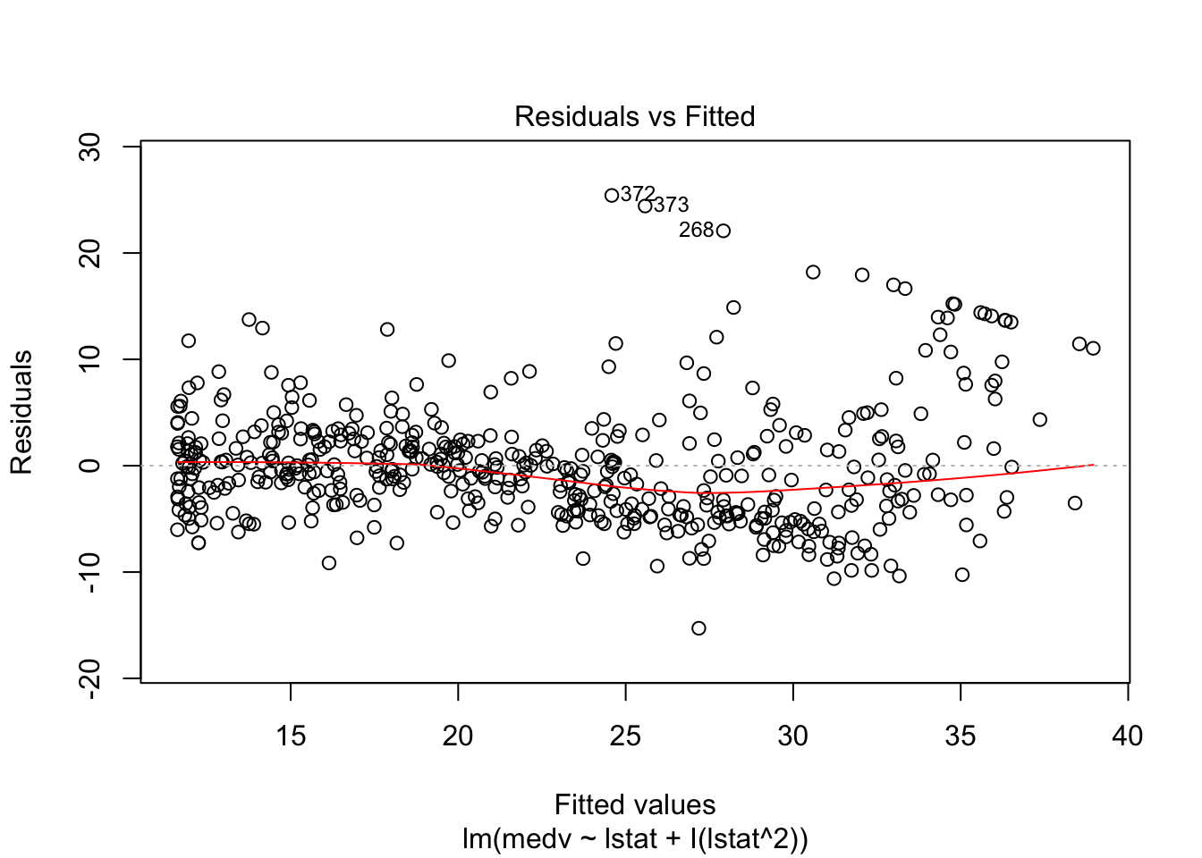

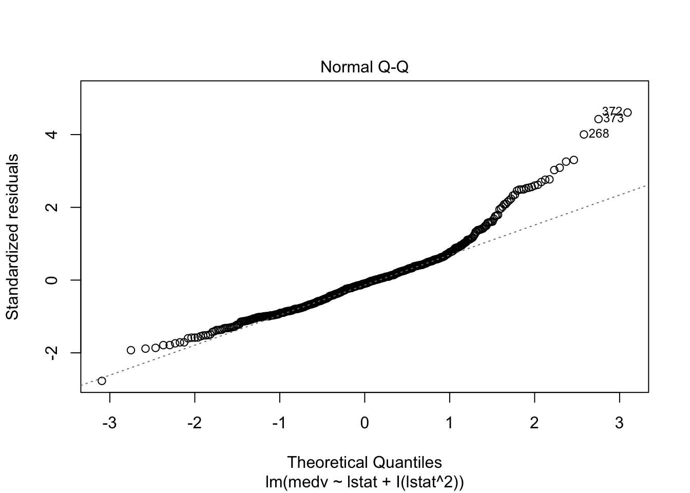
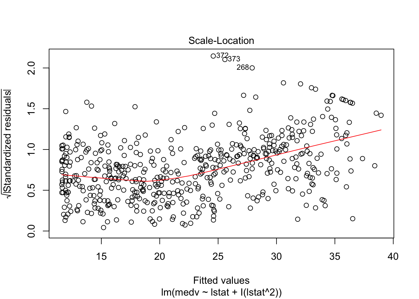
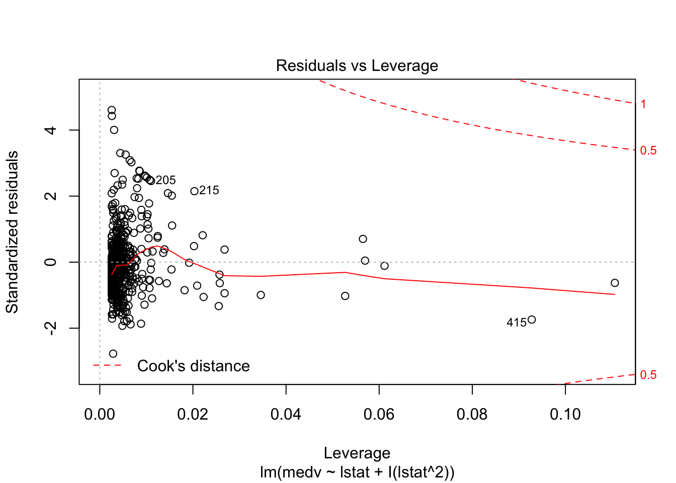
# Test if the model with a square is better than the simpler one:
anova(lm_fit, lm_fit_square)

## Analysis of Variance Table
## 
## Model 1: medv ~ lstat
## Model 2: medv ~ lstat + I(lstat^2)
##   Res.Df   RSS Df Sum of Sq     F                Pr(>F)    
## 1    504 19472                                             
## 2    503 15347  1    4125.1 135.2 < 0.00000000000000022 ***
## ---
## Signif. codes:  0 '***' 0.001 '**' 0.01 '*' 0.05 '.' 0.1 ' ' 1

# We can include higher polynomials:
summary(lm(medv ~ poly(lstat, 10), data = Boston))

## 
## Call:
## lm(formula = medv ~ poly(lstat, 10), data = Boston)
## 
## Residuals:
##      Min       1Q   Median       3Q      Max 
## -14.5340  -3.0286  -0.7507   2.0437  26.4738 
## 
## Coefficients:
##                    Estimate Std. Error t value             Pr(>|t|)    
## (Intercept)         22.5328     0.2311  97.488 < 0.0000000000000002 ***
## poly(lstat, 10)1  -152.4595     5.1993 -29.323 < 0.0000000000000002 ***
## poly(lstat, 10)2    64.2272     5.1993  12.353 < 0.0000000000000002 ***
## poly(lstat, 10)3   -27.0511     5.1993  -5.203          0.000000288 ***
## poly(lstat, 10)4    25.4517     5.1993   4.895          0.000001331 ***
## poly(lstat, 10)5   -19.2524     5.1993  -3.703             0.000237 ***
## poly(lstat, 10)6     6.5088     5.1993   1.252             0.211211    
## poly(lstat, 10)7     1.9416     5.1993   0.373             0.708977    
## poly(lstat, 10)8    -6.7299     5.1993  -1.294             0.196133    
## poly(lstat, 10)9     8.4168     5.1993   1.619             0.106116    
## poly(lstat, 10)10   -7.3351     5.1993  -1.411             0.158930    
## ---
## Signif. codes:  0 '***' 0.001 '**' 0.01 '*' 0.05 '.' 0.1 ' ' 1
## 
## Residual standard error: 5.199 on 495 degrees of freedom
## Multiple R-squared:  0.6867, Adjusted R-squared:  0.6804 
## F-statistic: 108.5 on 10 and 495 DF,  p-value: < 0.00000000000000022

# As we can see up to the 5th power all are statistically significant!

# We can also include different functions:
summary(lm(medv ~ log(lstat), data = Boston))

## 
## Call:
## lm(formula = medv ~ log(lstat), data = Boston)
## 
## Residuals:
##      Min       1Q   Median       3Q      Max 
## -14.4599  -3.5006  -0.6686   2.1688  26.0129 
## 
## Coefficients:
##             Estimate Std. Error t value            Pr(>|t|)    
## (Intercept)  52.1248     0.9652   54.00 <0.0000000000000002 ***
## log(lstat)  -12.4810     0.3946  -31.63 <0.0000000000000002 ***
## ---
## Signif. codes:  0 '***' 0.001 '**' 0.01 '*' 0.05 '.' 0.1 ' ' 1
## 
## Residual standard error: 5.329 on 504 degrees of freedom
## Multiple R-squared:  0.6649, Adjusted R-squared:  0.6643 
## F-statistic:  1000 on 1 and 504 DF,  p-value: < 0.00000000000000022

R for data science chapter 25: Many Models

This is beyond the scope of what we teach, but you might find it very useful in practice:

# We will be using the modelr and gapminder libraries for this part
gapminder

## # A tibble: 1,704 x 6
##    country     continent  year lifeExp      pop gdpPercap
##    <fct>       <fct>     <int>   <dbl>    <int>     <dbl>
##  1 Afghanistan Asia       1952    28.8  8425333      779.
##  2 Afghanistan Asia       1957    30.3  9240934      821.
##  3 Afghanistan Asia       1962    32.0 10267083      853.
##  4 Afghanistan Asia       1967    34.0 11537966      836.
##  5 Afghanistan Asia       1972    36.1 13079460      740.
##  6 Afghanistan Asia       1977    38.4 14880372      786.
##  7 Afghanistan Asia       1982    39.9 12881816      978.
##  8 Afghanistan Asia       1987    40.8 13867957      852.
##  9 Afghanistan Asia       1992    41.7 16317921      649.
## 10 Afghanistan Asia       1997    41.8 22227415      635.
## # … with 1,694 more rows

# plot life expectancy over time by country
gapminder %>% 
  ggplot(aes(x = year, y = lifeExp, group = country)) +
    geom_line(alpha = 1/3)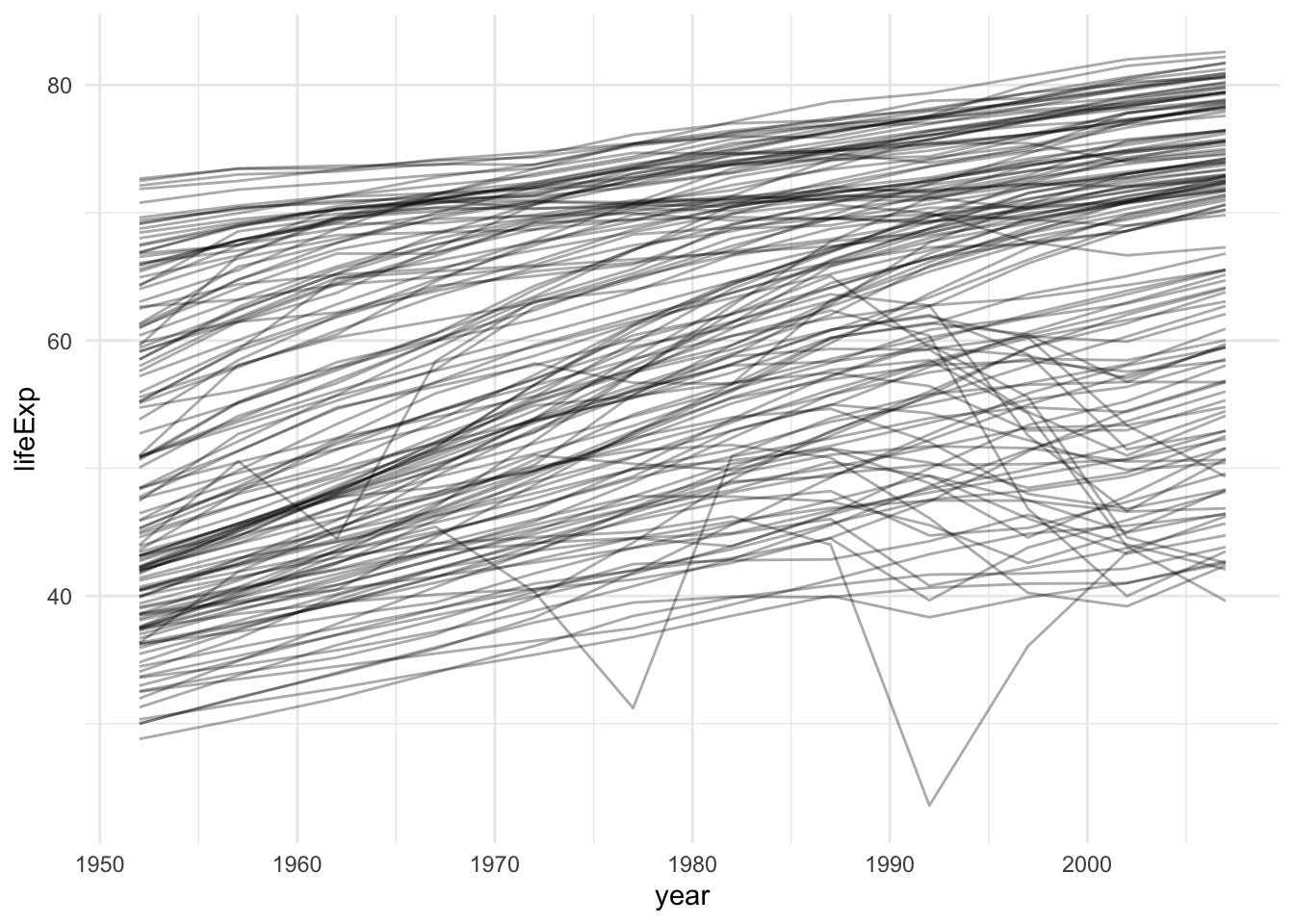

It’s really hard to see what is going on!

Solution: Do it by country and nest all of the results in a table

# Create a tibble that separates each country's data into a separate tibble:
by_country <- gapminder %>% 
  group_by(country, continent) %>% 
  nest()
# We group by country and continent since for a country continent is fixed and we 
# want to carry on another variable

# View the data:
by_country

## # A tibble: 142 x 3
## # Groups:   country, continent [710]
##    country     continent           data
##    <fct>       <fct>     <list<df[,4]>>
##  1 Afghanistan Asia            [12 × 4]
##  2 Albania     Europe          [12 × 4]
##  3 Algeria     Africa          [12 × 4]
##  4 Angola      Africa          [12 × 4]
##  5 Argentina   Americas        [12 × 4]
##  6 Australia   Oceania         [12 × 4]
##  7 Austria     Europe          [12 × 4]
##  8 Bahrain     Asia            [12 × 4]
##  9 Bangladesh  Asia            [12 × 4]
## 10 Belgium     Europe          [12 × 4]
## # … with 132 more rows

In this dataset each row is the complete dataset for a country, instead of being just one of the observations.

Now we want to fit a separate model for each of those rows:

# First we define the function that creates a linear model:
country_model <- function(df) {
  lm(lifeExp ~ year, data = df)
}

# Then we can abuse the purrr package to apply that function to each of 
# the elements of a list:
by_country <- by_country %>%
    mutate(model = map(data, country_model))

## mutate (grouped): new variable 'model' with 142 unique values and 0% NA

# Now the column "model" in the by_country tibble contains all of the linear models we just fit!
by_country

## # A tibble: 142 x 4
## # Groups:   country, continent [710]
##    country     continent           data model 
##    <fct>       <fct>     <list<df[,4]>> <list>
##  1 Afghanistan Asia            [12 × 4] <lm>  
##  2 Albania     Europe          [12 × 4] <lm>  
##  3 Algeria     Africa          [12 × 4] <lm>  
##  4 Angola      Africa          [12 × 4] <lm>  
##  5 Argentina   Americas        [12 × 4] <lm>  
##  6 Australia   Oceania         [12 × 4] <lm>  
##  7 Austria     Europe          [12 × 4] <lm>  
##  8 Bahrain     Asia            [12 × 4] <lm>  
##  9 Bangladesh  Asia            [12 × 4] <lm>  
## 10 Belgium     Europe          [12 × 4] <lm>  
## # … with 132 more rows

Now we want to look at the residuals, acessing models stored within tibbles is a hassle, so we can unnest the models:

by_country <- by_country %>% 
  mutate(
    resids = map2(data, model, add_residuals)
  )

## mutate (grouped): new variable 'resids' with 142 unique values and 0% NA

# Let's unnest the residuals:
resids <- unnest(by_country, resids)

# Plot the residuals:
resids %>% 
  ggplot(aes(year, resid)) +
    geom_line(aes(group = country), alpha = 1 / 3) + 
    geom_smooth(se = FALSE)

## `geom_smooth()` using method = 'gam' and formula 'y ~ s(x, bs = "cs")'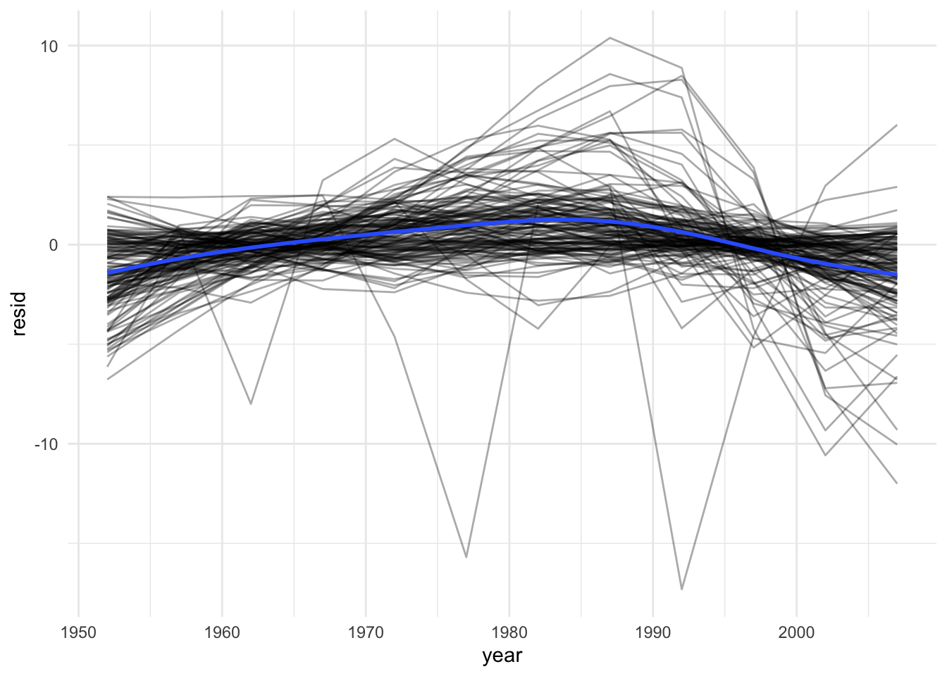

# Let's see the residuals by continent:
resids %>% 
  ggplot(aes(year, resid, group = country)) +
    geom_line(alpha = 1 / 3) + 
    facet_wrap(~continent)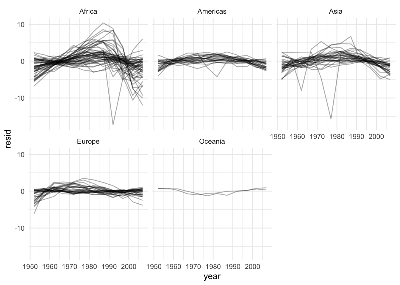

Week 5

Principal Component Analysis

With thanks to Alex Stringer for teaching me this in STA414

Motivation:

Sometimes we are given a dataset containing a much larger number of features than what we like for analysis. (We will see this specifically in lab 3). Principal Component Analysis is one way of reducing the number of features while maintaining as much information about the original data as possible.

Procedure:

Given a $n$ datapoints with $p$ features each, PCA tries to find a low-dimensional $d < p$ factorization of the data matrix $X$ that preserves the maximum possible variance.

\[ X = UZ \] \[ X \in \mathbb{R}^{n \times p} \] \[ Z \in \mathbb{R}^{d \times p} \] \[ U \in \mathbb{R}^{n \times d} \]

We estimate $U$ from the data, and call the associated $Z$ the principal components of $X$.

PCA is thus states as follows:

for $j = 1, ..., d$

\[ \mathbf{u}_j = argmax(Var(\mathbf{u}^T\mathbf{x})) = argmax(\mathbf{u}^T\mathbf{Su}) \]

subject to:

\[ \mathbf{u}^T\mathbf{u} = 1 ,~~ \text{and } ~ \mathbf{u} \perp \mathbf{u}_k ~~ \text{for} ~~ k < j \]

Where S is the sample covariance matrix: \[ \mathbf{S} = \frac{1}{n}\sum_{i = 1}^{n}{(\mathbf{x_i} - \mathbf{\bar{x}})(\mathbf{x_i} - \mathbf{\bar{x}}) ^T} \]

Using lagrange multipliers we see the solution to the above problem must satisfy:

\[ \mathbf{S}\mathbf{u}_1 = \lambda \mathbf{u}_1 \] Which means that $\mathbf{u}_1$ is an eigenvector of S with the eigenvalue $\lambda$.

By definition of the problem $\lambda$ must be the largest eigenvalue. This is since it doesn’t the second constraint (as there is no previously selected vectors)

Solving this constrained optimization problem gives us an orthonormal basis where the basis vectors point in the directions of the principal axes of the sample covariance matrix, in decreasing order of length.

It’s equivalent to the rotation in the original input space!

We then proceed to “chop off” the $d-p$ dimensions with least variance. And call this the basis for our $d$ dimensional space.

So, the solution to the PCA problem is:

Choose $\mathbf{u}_j$ to be normalized eigenvector of $\mathbf{S}$ corresponding to the $j$-th highest eigenvalue.
Choose $\mathbf{U}$ to be the matrix of orthonormal eigenvectors of S, so that $\mathbf{U}^T\mathbf{U} = \mathbf{I}$
Then $\mathbf{Z} = \mathbf{XU}^T$.
Keep only the first d columns of $\mathbf{Z}$ and the corresponding $d \times d$ submatrix of $\mathbf{U}$
Reconstruct the data as $\mathbf{X}^* = \mathbf{Z}^*\mathbf{U}^*$

Lab 1: PCA

# See variable names
colnames(USArrests)

## [1] "Murder"   "Assault"  "UrbanPop" "Rape"

# Display means of each row
USArrests %>% summarize_all(funs(mean))

## summarize_all: now one row and 4 columns, ungrouped

##   Murder Assault UrbanPop   Rape
## 1  7.788  170.76    65.54 21.232

# Display means and variances of each row
USArrests %>% summarize_all(.funs = c(Mean = mean, Variance = var))

## summarize_all: now one row and 8 columns, ungrouped

##   Murder_Mean Assault_Mean UrbanPop_Mean Rape_Mean Murder_Variance
## 1       7.788       170.76         65.54    21.232        18.97047
##   Assault_Variance UrbanPop_Variance Rape_Variance
## 1         6945.166          209.5188      87.72916

There is a built-in function in R to do the principal component analysis:

It automatically scales the data to have the mean of 0

There is an added parameter scale which will also scale the standard deviation to 1.

In general there are at most $min(n-1,p)$ informative principal components.

# compute the PCA
pca_out = prcomp(USArrests , scale = TRUE)
# output the rotation matrix
pca_out$rotation

##                 PC1        PC2        PC3         PC4
## Murder   -0.5358995  0.4181809 -0.3412327  0.64922780
## Assault  -0.5831836  0.1879856 -0.2681484 -0.74340748
## UrbanPop -0.2781909 -0.8728062 -0.3780158  0.13387773
## Rape     -0.5434321 -0.1673186  0.8177779  0.08902432

# output the reconstructed data in the new coordinates:
pca_out$x

##                        PC1         PC2         PC3          PC4
## Alabama        -0.97566045  1.12200121 -0.43980366  0.154696581
## Alaska         -1.93053788  1.06242692  2.01950027 -0.434175454
## Arizona        -1.74544285 -0.73845954  0.05423025 -0.826264240
## Arkansas        0.13999894  1.10854226  0.11342217 -0.180973554
## California     -2.49861285 -1.52742672  0.59254100 -0.338559240
## Colorado       -1.49934074 -0.97762966  1.08400162  0.001450164
## Connecticut     1.34499236 -1.07798362 -0.63679250 -0.117278736
## Delaware       -0.04722981 -0.32208890 -0.71141032 -0.873113315
## Florida        -2.98275967  0.03883425 -0.57103206 -0.095317042
## Georgia        -1.62280742  1.26608838 -0.33901818  1.065974459
## Hawaii          0.90348448 -1.55467609  0.05027151  0.893733198
## Idaho           1.62331903  0.20885253  0.25719021 -0.494087852
## Illinois       -1.36505197 -0.67498834 -0.67068647 -0.120794916
## Indiana         0.50038122 -0.15003926  0.22576277  0.420397595
## Iowa            2.23099579 -0.10300828  0.16291036  0.017379470
## Kansas          0.78887206 -0.26744941  0.02529648  0.204421034
## Kentucky        0.74331256  0.94880748 -0.02808429  0.663817237
## Louisiana      -1.54909076  0.86230011 -0.77560598  0.450157791
## Maine           2.37274014  0.37260865 -0.06502225 -0.327138529
## Maryland       -1.74564663  0.42335704 -0.15566968 -0.553450589
## Massachusetts   0.48128007 -1.45967706 -0.60337172 -0.177793902
## Michigan       -2.08725025 -0.15383500  0.38100046  0.101343128
## Minnesota       1.67566951 -0.62590670  0.15153200  0.066640316
## Mississippi    -0.98647919  2.36973712 -0.73336290  0.213342049
## Missouri       -0.68978426 -0.26070794  0.37365033  0.223554811
## Montana         1.17353751  0.53147851  0.24440796  0.122498555
## Nebraska        1.25291625 -0.19200440  0.17380930  0.015733156
## Nevada         -2.84550542 -0.76780502  1.15168793  0.311354436
## New Hampshire   2.35995585 -0.01790055  0.03648498 -0.032804291
## New Jersey     -0.17974128 -1.43493745 -0.75677041  0.240936580
## New Mexico     -1.96012351  0.14141308  0.18184598 -0.336121113
## New York       -1.66566662 -0.81491072 -0.63661186 -0.013348844
## North Carolina -1.11208808  2.20561081 -0.85489245 -0.944789648
## North Dakota    2.96215223  0.59309738  0.29824930 -0.251434626
## Ohio            0.22369436 -0.73477837 -0.03082616  0.469152817
## Oklahoma        0.30864928 -0.28496113 -0.01515592  0.010228476
## Oregon         -0.05852787 -0.53596999  0.93038718 -0.235390872
## Pennsylvania    0.87948680 -0.56536050 -0.39660218  0.355452378
## Rhode Island    0.85509072 -1.47698328 -1.35617705 -0.607402746
## South Carolina -1.30744986  1.91397297 -0.29751723 -0.130145378
## South Dakota    1.96779669  0.81506822  0.38538073 -0.108470512
## Tennessee      -0.98969377  0.85160534  0.18619262  0.646302674
## Texas          -1.34151838 -0.40833518 -0.48712332  0.636731051
## Utah            0.54503180 -1.45671524  0.29077592 -0.081486749
## Vermont         2.77325613  1.38819435  0.83280797 -0.143433697
## Virginia        0.09536670  0.19772785  0.01159482  0.209246429
## Washington      0.21472339 -0.96037394  0.61859067 -0.218628161
## West Virginia   2.08739306  1.41052627  0.10372163  0.130583080
## Wisconsin       2.05881199 -0.60512507 -0.13746933  0.182253407
## Wyoming         0.62310061  0.31778662 -0.23824049 -0.164976866

# To get the variance explained by each of the prinicpal components we take the 
# square of the std deviation:
pca_var <- pca_out$sdev^2
pca_var

## [1] 2.4802416 0.9897652 0.3565632 0.1734301

# To get the proportion of variance explained we just need to divide by the sum:
pca_varprop <- pca_var / sum(pca_var)
pca_varprop

## [1] 0.62006039 0.24744129 0.08914080 0.04335752

# Plots using base R:
plot(pca_varprop , xlab = " Principal Component ",
     ylab = "Proportion of Variance Explained ",
     ylim = c(0,1), type = "b")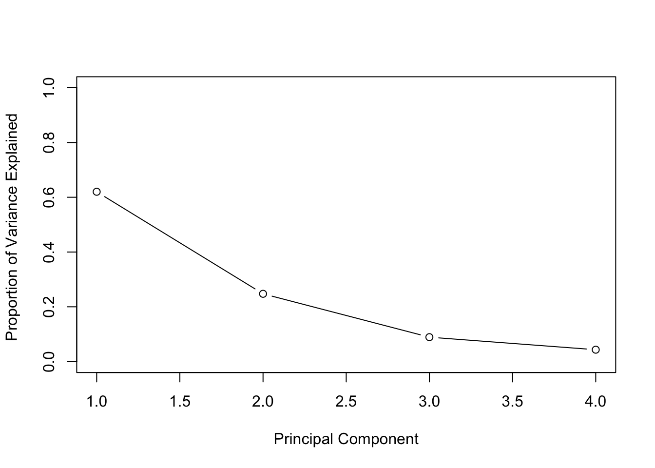

plot(cumsum(pca_varprop), xlab = "Principal Component ",
     ylab = "Cumulative Proportion of Variance Explained",
     ylim = c(0,1), type = "b")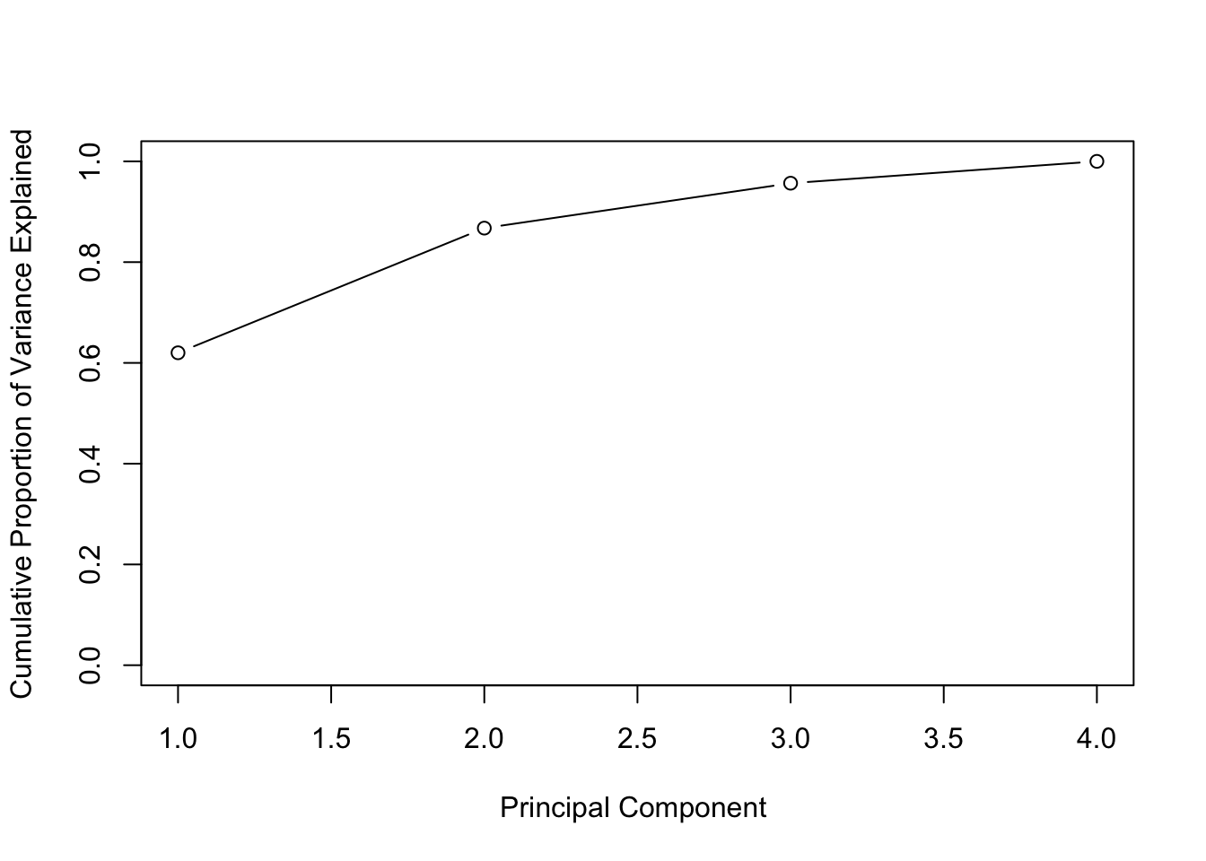

# Plots using ggplot:
## Create the combined dataset:
df <- tibble(PCA = 1:4, VarianceProportion = pca_varprop)

ggplot(data = df, aes(x = PCA, y = VarianceProportion)) +
    geom_line() +
    geom_point() +
    labs(x = "Principal Component", y = "Proportion of Variance Explained") +
    geom_text(aes(label = round(VarianceProportion,2)), vjust = -1) +
    scale_y_continuous(limits = c(0, 1))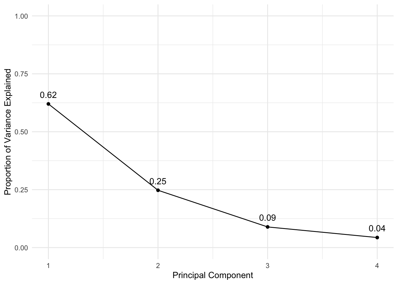

ggplot(data = df, aes(x = PCA, y = cumsum(VarianceProportion))) +
    geom_line() +
    geom_point() +
    labs(x = "Principal Component", y = "Cumulative Proportion of Variance Explained") +
    geom_text(aes(label = round(cumsum(VarianceProportion),2)), vjust = 2) +
    scale_y_continuous(limits = c(0, 1))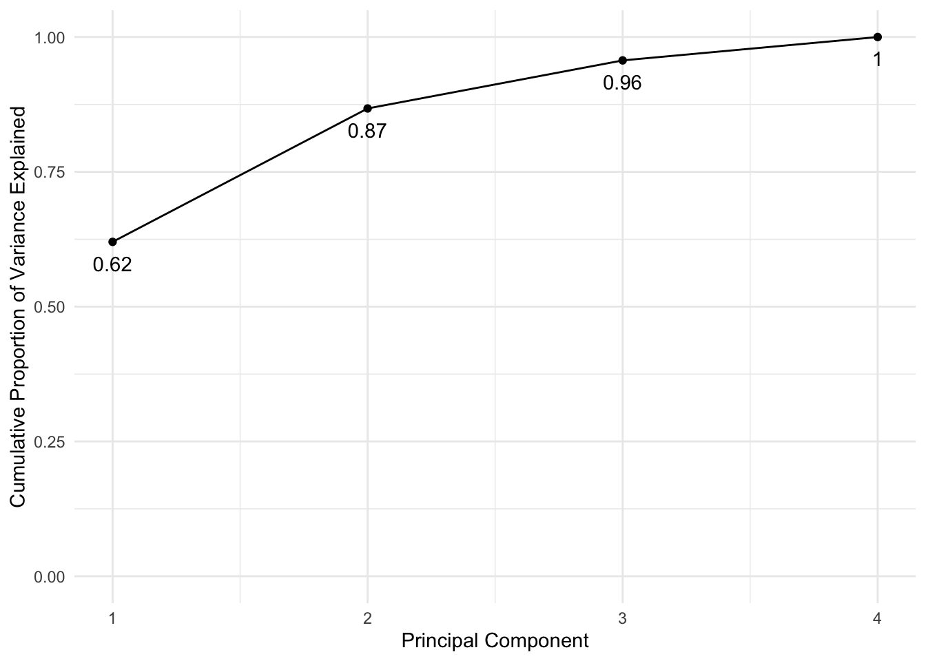

# standardize all the variables
USArrests_std <- USArrests %>% mutate_all(.funs = (scale))

## mutate_all: changed 50 values (100%) of 'Murder' (0 new NA)

##             converted 'Assault' from integer to double (0 new NA)

##             converted 'UrbanPop' from integer to double (0 new NA)

##             changed 50 values (100%) of 'Rape' (0 new NA)

varcov_matrix <- cor(USArrests_std)
varcov_matrix

##              Murder   Assault   UrbanPop      Rape
## Murder   1.00000000 0.8018733 0.06957262 0.5635788
## Assault  0.80187331 1.0000000 0.25887170 0.6652412
## UrbanPop 0.06957262 0.2588717 1.00000000 0.4113412
## Rape     0.56357883 0.6652412 0.41134124 1.0000000

# look at the eigenvectors and eigenvalues of the var cov matrix
e <- eigen(varcov_matrix)
e

## eigen() decomposition
## $values
## [1] 2.4802416 0.9897652 0.3565632 0.1734301
## 
## $vectors
##            [,1]       [,2]       [,3]        [,4]
## [1,] -0.5358995  0.4181809 -0.3412327  0.64922780
## [2,] -0.5831836  0.1879856 -0.2681484 -0.74340748
## [3,] -0.2781909 -0.8728062 -0.3780158  0.13387773
## [4,] -0.5434321 -0.1673186  0.8177779  0.08902432

# Compute the eigenvector transformation

for (i in 1:length(names(USArrests_std))) {
    assign(paste0("PC", i), 
    as.vector(USArrests_std$Murder * e$vectors[1,i] +
    USArrests_std$Assault * e$vectors[2,i] + 
    USArrests_std$UrbanPop * e$vectors[3,i] +
    USArrests_std$Rape * e$vectors[4,i]))
}

manual_PCA <- tibble(PC1 = PC1, PC2 = PC2, PC3 = PC3, PC4 = PC4)
auto_PCA <- as.tibble(pca_out$x)

## Warning: `as.tibble()` is deprecated, use `as_tibble()` (but mind the new semantics).
## This warning is displayed once per session.

difference = manual_PCA - auto_PCA
difference

##                          PC1                       PC2
## 1  -0.0000000000000005551115 -0.0000000000000008881784
## 2   0.0000000000000006661338 -0.0000000000000008881784
## 3   0.0000000000000011102230 -0.0000000000000019984014
## 4  -0.0000000000000008326673  0.0000000000000002220446
## 5   0.0000000000000022204460 -0.0000000000000024424907
## 6   0.0000000000000017763568 -0.0000000000000011102230
## 7   0.0000000000000000000000  0.0000000000000008881784
## 8   0.0000000000000001665335 -0.0000000000000004996004
## 9   0.0000000000000013322676 -0.0000000000000030808689
## 10 -0.0000000000000002220446 -0.0000000000000013322676
## 11  0.0000000000000006661338  0.0000000000000006661338
## 12 -0.0000000000000008881784  0.0000000000000016375790
## 13  0.0000000000000006661338 -0.0000000000000016653345
## 14 -0.0000000000000002220446  0.0000000000000006106227
## 15 -0.0000000000000004440892  0.0000000000000021371793
## 16 -0.0000000000000002220446  0.0000000000000007771561
## 17 -0.0000000000000011102230  0.0000000000000009992007
## 18  0.0000000000000000000000 -0.0000000000000015543122
## 19 -0.0000000000000008881784  0.0000000000000024424907
## 20  0.0000000000000004440892 -0.0000000000000017763568
## 21  0.0000000000000005551115  0.0000000000000002220446
## 22  0.0000000000000004440892 -0.0000000000000019151347
## 23  0.0000000000000000000000  0.0000000000000016653345
## 24 -0.0000000000000015543122 -0.0000000000000008881784
## 25  0.0000000000000005551115 -0.0000000000000004996004
## 26 -0.0000000000000008881784  0.0000000000000013322676
## 27 -0.0000000000000002220446  0.0000000000000013045121
## 28  0.0000000000000017763568 -0.0000000000000024424907
## 29 -0.0000000000000008881784  0.0000000000000025257574
## 30  0.0000000000000008881784 -0.0000000000000006661338
## 31  0.0000000000000008881784 -0.0000000000000019151347
## 32  0.0000000000000015543122 -0.0000000000000019984014
## 33 -0.0000000000000015543122 -0.0000000000000013322676
## 34 -0.0000000000000017763568  0.0000000000000029976022
## 35  0.0000000000000003608225  0.0000000000000000000000
## 36  0.0000000000000001665335  0.0000000000000002775558
## 37  0.0000000000000006106227  0.0000000000000001110223
## 38 -0.0000000000000002220446  0.0000000000000007771561
## 39  0.0000000000000004440892  0.0000000000000002220446
## 40 -0.0000000000000008881784 -0.0000000000000008881784
## 41 -0.0000000000000011102230  0.0000000000000022204460
## 42 -0.0000000000000002220446 -0.0000000000000005551115
## 43  0.0000000000000006661338 -0.0000000000000014432899
## 44  0.0000000000000008881784  0.0000000000000004440892
## 45 -0.0000000000000022204460  0.0000000000000031086245
## 46 -0.0000000000000002081668  0.0000000000000001665335
## 47  0.0000000000000008326673  0.0000000000000002220446
## 48 -0.0000000000000017763568  0.0000000000000019984014
## 49 -0.0000000000000004440892  0.0000000000000017763568
## 50 -0.0000000000000005551115  0.0000000000000004996004
##                           PC3                        PC4
## 1  -0.00000000000000033306691 -0.00000000000000099920072
## 2   0.00000000000000044408921  0.00000000000000194289029
## 3   0.00000000000000155431223  0.00000000000000066613381
## 4  -0.00000000000000011102230 -0.00000000000000038857806
## 5   0.00000000000000133226763  0.00000000000000166533454
## 6   0.00000000000000022204460  0.00000000000000185962357
## 7   0.00000000000000022204460 -0.00000000000000015265567
## 8   0.00000000000000111022302 -0.00000000000000055511151
## 9   0.00000000000000088817842 -0.00000000000000034694470
## 10 -0.00000000000000111022302 -0.00000000000000066613381
## 11 -0.00000000000000083266727  0.00000000000000066613381
## 12  0.00000000000000022204460  0.00000000000000005551115
## 13  0.00000000000000066613381 -0.00000000000000036082248
## 14 -0.00000000000000055511151  0.00000000000000033306691
## 15 -0.00000000000000066613381  0.00000000000000009714451
## 16 -0.00000000000000038857806  0.00000000000000008326673
## 17 -0.00000000000000111022302 -0.00000000000000055511151
## 18 -0.00000000000000044408921 -0.00000000000000111022302
## 19 -0.00000000000000022204460 -0.00000000000000044408921
## 20  0.00000000000000088817842 -0.00000000000000044408921
## 21  0.00000000000000044408921  0.00000000000000000000000
## 22  0.00000000000000033306691  0.00000000000000069388939
## 23 -0.00000000000000033306691  0.00000000000000029143354
## 24 -0.00000000000000066613381 -0.00000000000000188737914
## 25 -0.00000000000000005551115  0.00000000000000061062266
## 26 -0.00000000000000044408921 -0.00000000000000009714451
## 27 -0.00000000000000011102230  0.00000000000000024286129
## 28  0.00000000000000022204460  0.00000000000000177635684
## 29 -0.00000000000000044408921 -0.00000000000000011102230
## 30  0.00000000000000022204460 -0.00000000000000016653345
## 31  0.00000000000000077715612  0.00000000000000038857806
## 32  0.00000000000000066613381 -0.00000000000000022898350
## 33  0.00000000000000099920072 -0.00000000000000188737914
## 34 -0.00000000000000044408921 -0.00000000000000022204460
## 35 -0.00000000000000041633363  0.00000000000000022204460
## 36 -0.00000000000000002775558  0.00000000000000011102230
## 37  0.00000000000000033306691  0.00000000000000138777878
## 38 -0.00000000000000044408921 -0.00000000000000033306691
## 39  0.00000000000000111022302 -0.00000000000000088817842
## 40  0.00000000000000005551115 -0.00000000000000108246745
## 41 -0.00000000000000044408921 -0.00000000000000005551115
## 42 -0.00000000000000077715612 -0.00000000000000011102230
## 43 -0.00000000000000033306691 -0.00000000000000033306691
## 44  0.00000000000000022204460  0.00000000000000090205621
## 45 -0.00000000000000088817842  0.00000000000000030531133
## 46 -0.00000000000000029837244 -0.00000000000000008326673
## 47  0.00000000000000033306691  0.00000000000000111022302
## 48 -0.00000000000000088817842 -0.00000000000000072164497
## 49 -0.00000000000000055511151 -0.00000000000000005551115
## 50  0.00000000000000000000000 -0.00000000000000047184479

Lab 3: PCA and Clustering

# Data Load
nci_labs <- NCI60$labs
nci_data <- NCI60$data

# Combine
nci <- as.tibble(nci_data)
nci$labels <- nci_labs

# It's a large dataset! 
dim(nci)

## [1]   64 6831

# Let's see what are the possible labels
unique(nci$labels)

##  [1] "CNS"         "RENAL"       "BREAST"      "NSCLC"       "UNKNOWN"    
##  [6] "OVARIAN"     "MELANOMA"    "PROSTATE"    "LEUKEMIA"    "K562B-repro"
## [11] "K562A-repro" "COLON"       "MCF7A-repro" "MCF7D-repro"

# Let's see how many of each label:
nci %>% group_by(labels) %>% summarize(n())

## group_by: one grouping variable (labels)

## summarize: now 14 rows and 2 columns, ungrouped

## # A tibble: 14 x 2
##    labels      `n()`
##    <chr>       <int>
##  1 BREAST          7
##  2 CNS             5
##  3 COLON           7
##  4 K562A-repro     1
##  5 K562B-repro     1
##  6 LEUKEMIA        6
##  7 MCF7A-repro     1
##  8 MCF7D-repro     1
##  9 MELANOMA        8
## 10 NSCLC           9
## 11 OVARIAN         6
## 12 PROSTATE        2
## 13 RENAL           9
## 14 UNKNOWN         1

# Not very many data points, with a lot of features!

Are all of those features really necessary? Let’s try doing PCA and seeing what proportion of variance can be explained by taking just a few:

# I don't want to rescale the labels (which are not numerical in the first place!)
nci_pca <- nci_data %>% prcomp(scale = TRUE)

# Since we will be plotting this data, we would like a function that assigns 
# a color based on the value of the label to each of the datapoints:

Colors = function(vec) {
    colors = rainbow(length(unique(vec)))
    return(colors[as.numeric(as.factor(vec))])
}

# Now let's plot the PCs 
par(mfrow = c(1,2))

# plot the first and second PC
plot(nci_pca$x[,1:2], col = Colors(nci_labs), pch = 19, xlab = "PC1",ylab = "PC2")
# plot the first and third PC
plot(nci_pca$x[,c(1,3)], col = Colors(nci_labs), pch = 19, xlab = "PC1", ylab = "PC3")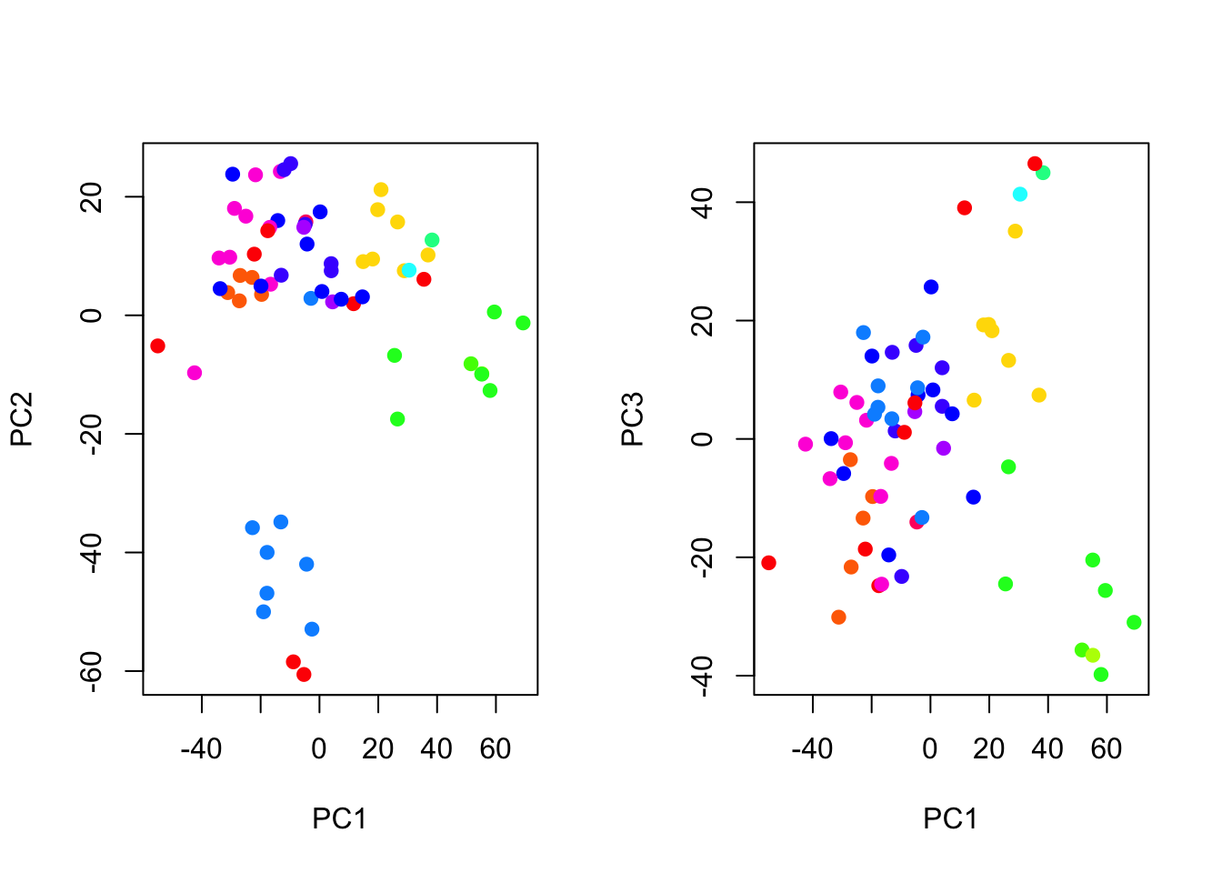

# Get back to regular plotting:
par(mfrow = c(1,1))

Now if we want to plot without having to write a function to assign colors each time, we can use ggplot:

# Save as tibble for convenience (you could probably get away with not doing this)
nci_pca_tb <- as.tibble(nci_pca$x)
# Add back the labels 
nci_pca_tb$labels <- nci$labels

# Plot (I'm dropping the argument names beyond this point)
ggplot(nci_pca_tb, aes(x = PC1, y = PC2, color = labels)) +
    geom_point()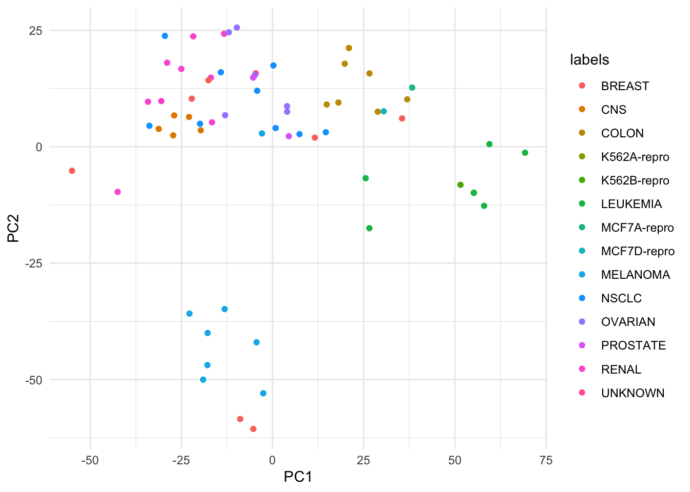

# Doesn't this look 100 times simpler to do ?
ggplot(nci_pca_tb, aes(x = PC1, y = PC3, color = labels)) +
    geom_point()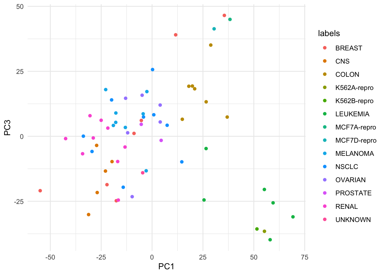

For this reason, beyond this point, I will be rewriting all of visualizations from the labs into tidyverse code and omit the base R code.

# Extract the variances
df <- tibble(PCA = 1:length(nci_pca$sdev), VarianceProportion = nci_pca$sdev^2 / sum(nci_pca$sdev^2))

# Plot just the variance explanation proportions
ggplot(data = df, aes(x = PCA, y = VarianceProportion)) +
    geom_line() +
    geom_point() +
    labs(x = "Principal Component", y = "Proportion of Variance Explained") +
    scale_y_continuous(limits = c(0, 1))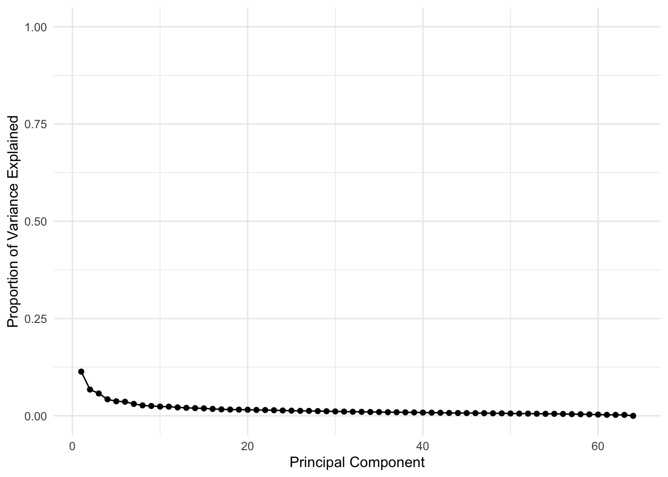

# Plot the cumulative variance explanation proportions 
ggplot(data = df, aes(x = PCA, y = cumsum(VarianceProportion))) +
    geom_line(color = if_else(cumsum(df$VarianceProportion) > 0.9, "red", "green")) +
    geom_point(color = if_else(cumsum(df$VarianceProportion) > 0.9, "red", "green")) +
    labs(x = "Principal Component", y = "Cumulative Proportion of Variance Explained") +
    scale_y_continuous(limits = c(0, 1)) +
    geom_line(y = 0.9)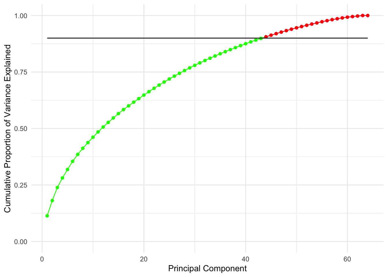

The line on the second plot shows at which point you can cut out to keep $90$% of variance ($90$% of information about data), which looks to be about 20 features.

Note that this is an improvent of an improvements since by just doing the PCA we have decreased the number of features from 6830 to 64 which is a 99.06% decrease, without losing much information!

Now let’s do some clustering to review what we were doing 2 weeks ago:

Again for simplicity of visualization I will be using the ggdendro package.

# Create a vector of types of Hierarchical clustering we covered
clustering_types <- c("complete", "average", "single")

# Perform HC in a loop and plotting
for (method in clustering_types) {
    # Good example of why %>% is a great operator and method chaining is important
    nci_data %>% # Take the data
    scale %>% # Rescale it
    dist %>%  # Create a distance matrix 
    hclust(method = method) %>% # Perform HC
    as.dendrogram %>% # Change type to dendrogram
    set("labels", nci_labs) %>% # Add the labels from the original data
    set("branches_k_color", k = 4) %>% # Split the tree into 4 classes and color
    set("labels_cex", 0.5) %>%
    plot(main = paste0(method," linkage"))
}

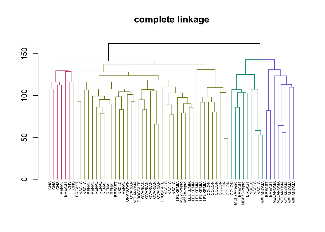
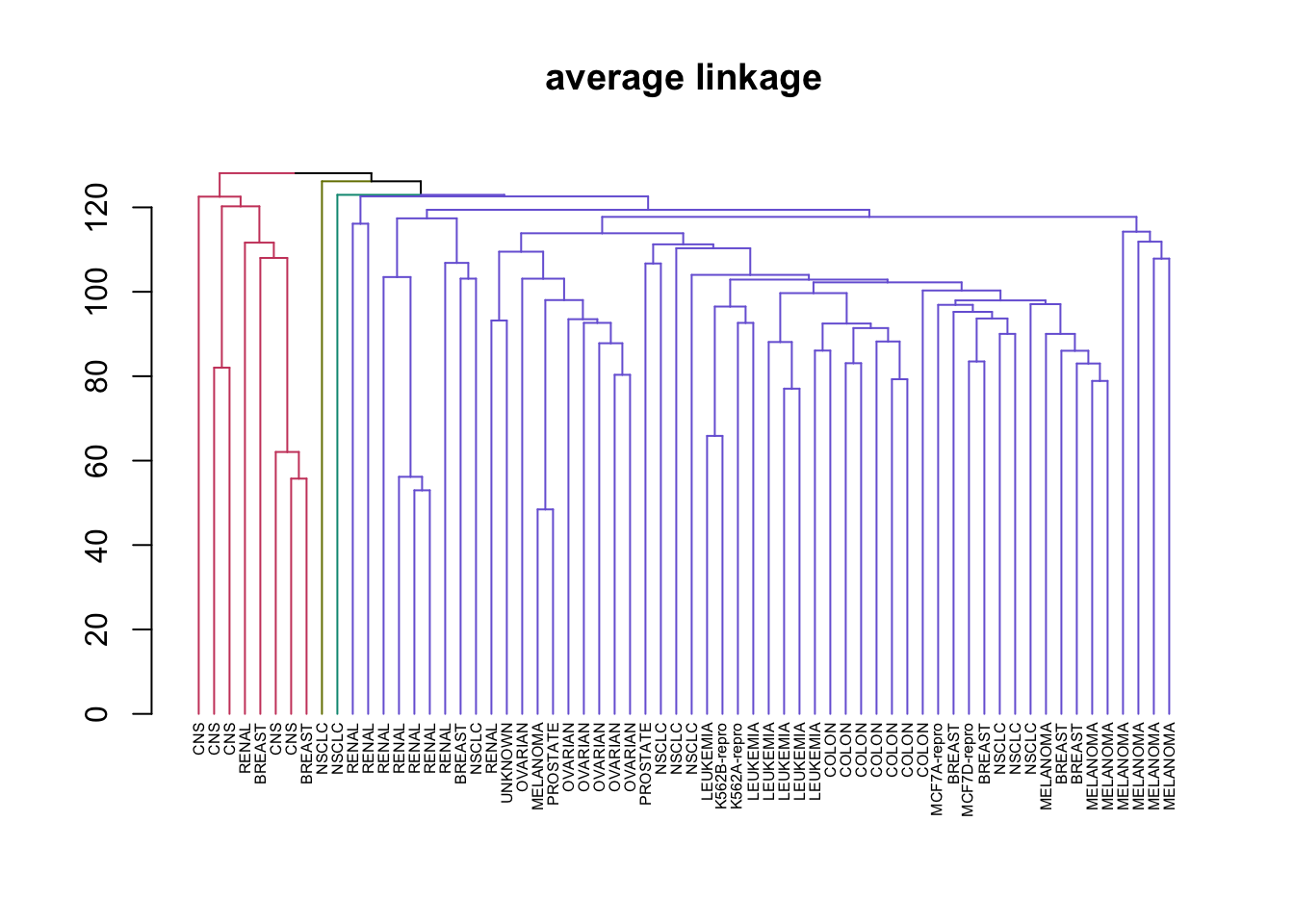
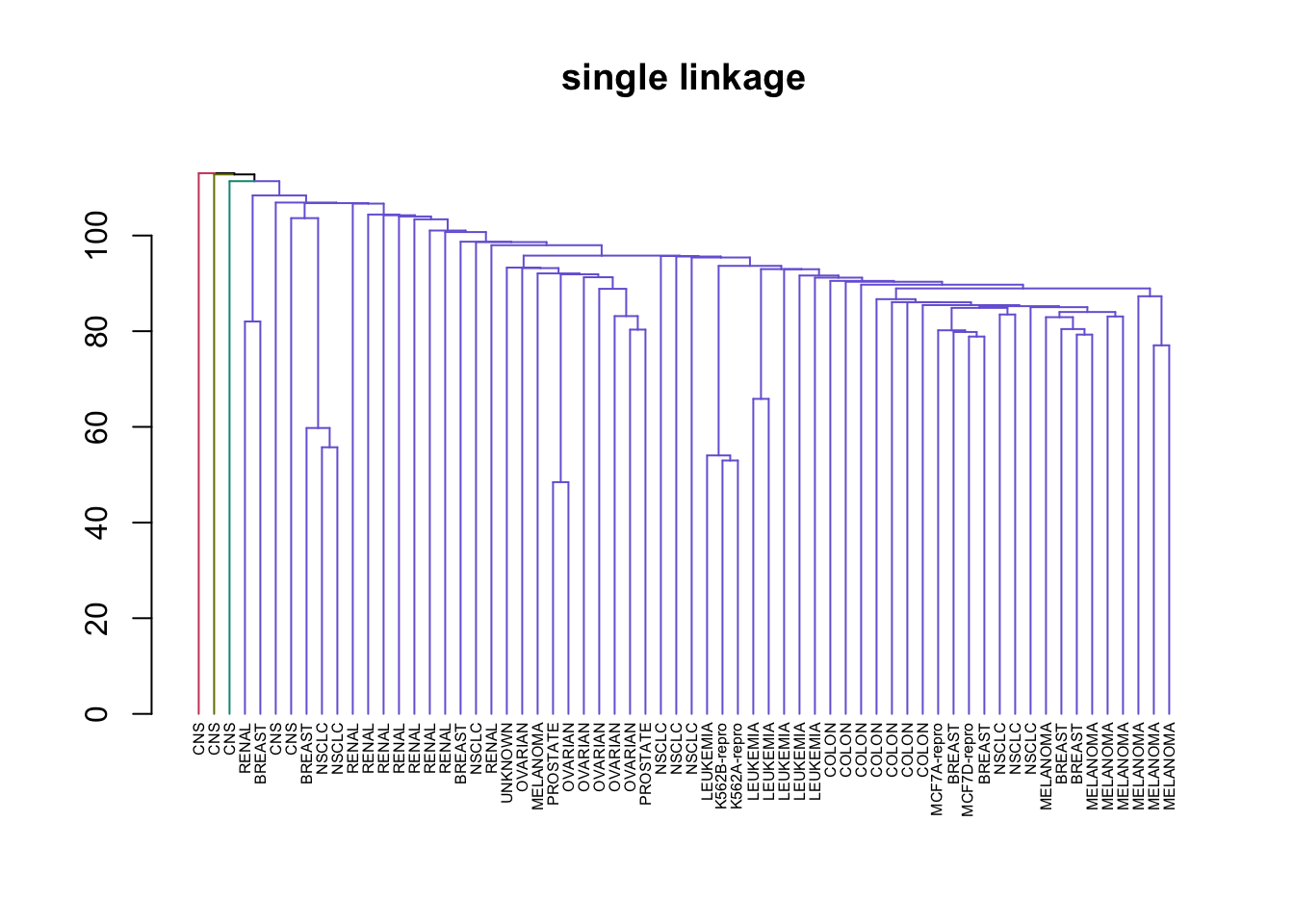
This illustrates just how different results can be for the types of HC we learned. Complete and average linkages usually result in similarily sized clusters, while Single linkage usually results in a single large cluster that has single leaves added to it at each step. Now let’s compare Complete Linkage with K-Means clustering

# Create the complete linkage clustering
cl_clusters <- nci_data %>% # Take the data
    scale %>% # Rescale it
    dist %>%  # Create a distance matrix 
    hclust(method = "complete") %>% # Perform HC
    cutree(k = 4) # cut 4 clusters

# Create the kmeans clustering
kmeans_clusters <- nci_data %>% # Take the data
    scale %>%
    kmeans(centers = 4, nstart = 20) # Perform K-Means for 4 clusters 20 times
    
# Create a comparison Table:
table(kmeans_clusters$cluster, cl_clusters)

##    cl_clusters
##      1  2  3  4
##   1 11  0  0  9
##   2 20  7  0  0
##   3  0  0  8  0
##   4  9  0  0  0

From this table we can see that cluster 4 in k-means is the same as cluster 3 in complete linkage, but the other clusters are a mixture. For example cluster 3 in k-means is a combination of 11 elements from cluster 1 in CL and 9 elements of cluster 4 in CL.

Question 3:

Question:

By modifying the argument used in the lecture, argue that the second principal component of a (centred) feature matrix $X$ should maximise the Rayleigh quotent of $X^TX$ over all vectors that are orthogonal to the first principal component and show that this implies that the second prinicipal component is the eigenvector of $X^TX$ that corresponds to the second largest eigenvalue.

Solution:

Solution adapted from Alin Morariu

The second principle component of a centred feature matrix $X$ should maximize Rayleigh’s quotient up to being orthogonal to the fist principle component.

Note, this argument is almost trivial once we understand that we can order our set of eigenvalues and combining this with the following notation:

\[ v_2 = \text{arg} \max_{v \in \mathbb{R}^p, v \perp v_1 } \frac{v^T X^T X v}{v^T v} \]

All that this is asking, is that we find the eigenvector that maximizes the quotient with respect to all vectors in $\mathbb{R}^p$ which are orthogonal to $v_1$. Furthermore, this corresponds to taking the second largest eignevalue from our ordered set. However, we will show this more rigorously using the argument made in class. We begin with the spectral decomposition of our feature matrix.

\[X^T X = UDU^T \text{ and define } Z = U^Tv \text{ where } v \in \mathbb{R}^p \]

\[ \Rightarrow v^T X^T X v = z^T D z = \sum_{i=1}^{p} \lambda_i z_i z_i^T \leq \sum_{i=1}^{p} \lambda_2 z_i z_i^T = \lambda_2 \sum_{i=1}^{p} z_i z_I^T = \lambda_2 v^T U^T U v\]

The inequality above turns into an equality in the case where $z_3 = z_4 = \ldots = z_p = 0$; otherwise we can say that $\lambda_2 \geq \lambda_i$ for $i \in \{3, 4, \ldots, p\}$ which in turn maximizes the quotient with respect to the constraints. This concludes the proof.

Question 4

Question:

An experiment was undertaken to exmaine differences in burritos made across Toronto. 400 burritos were purchased at commercial venues and four measurements were taken of each burrito: mass (in grams), length (in centimetres), sturdiness (scored from 1-10), and taste (scored from 1-10). The scaled sample covariance matrix was calculated and its four eigenvalues were found to be 14.1, 4.3, 1.2 and 0.4. The corresponding first and second eigenvectors were:

\[v_1^T = [0.39, 0.42, 0.44, 0.69]\] \[v_2^T = [0.40, 0.39, 0.42,−0.72]\]

What is the proportion of variance explained by the first two prinicple components?
Give an interpretation of the first two principal components
Suppose that the data were stored by recording the eigenvalues and eigenvectors together with the 400 values of the first and second principal components and the mean values for the original variables. How would you use this information reconstruct approximations to the original covariance matrix and the original data?

Solution:

Slightly modfied solution from Alin Morariu

Given: $\lambda^* = \{14.1, 4.3, 1.2, 0.4 \}$ , $v_1^T = [0.39, 0.42, 0.44, 0.69]$ , and $v_2^T = [0.40, 0.39, 0.42, -0.72]$

i)

We are asked to calculate the proportion of variance explained by the fist 2 principle components.

\[\text{proportion explained} = \frac{\sum_{i=1}^{2} \lambda_i }{\sum_{i=1}^{4} \lambda_i } = \frac{14.1 + 4.3}{14.1 + 4.3 + 1.2 + 0.4} = 0.92 \]

ii)

Interpreting the principle components:

First PC: Notice that each of the components have a positive coefficient we can say that heavier and longer burritos have a tendency to be tastier.

Second PC: Here we see that the component corresponding to taste has a negative coefficient which indicates that we have some burritos that are small, light, unsturdy and tasty OR large, heavy, sturdy, and bland (their scores would be equivalent).

iii)

Here we are tasked with reconstructing the variance-covariance matrix of the centred data based on our 2 eigenvectors, and 4 eigenvalues. We back out the desired result from the spectral decomposition of the variance-covariance matrix.

Since we only have the first two principal components we can only use the first two eigenvalues:

\[\hat{\Sigma} = \hat{U}\hat{D}\hat{U}^T = \sum_{i=1}^{2} \lambda_iv_i v_i^T = \lambda_1 v_1 v_1^T + \lambda_2 v_2 v_2^T \]

Note that we have all of the quantities specified above so now its a matter of plugging in the values and multiplying them together.

\[\hat{\Sigma} = \left( \begin{array}{cccc} 2.833 \\ 2.980 & 3.141 \\ 3.142 & 3.310 & 3.488 \\ 2.556 & 2.879 & 2.980 & 8.942 \end{array} \right) \]

Noting that $\hat{\Sigma}$ is symmetric we can fill in the rest.

Remember that we framed the original data as: \[ X = LU \] Where $U$ are the principal components and $L$ is the loading matrix. Thus to retrieve the original data we need to multiply our eigenvectors by our loading factors matrix to get estimates of mean corrected data.

\[ x_i^T = \begin{pmatrix} l_1 & l_2 \end{pmatrix} \begin{pmatrix} v_1^T\\ v_2^T \end{pmatrix} = \begin{pmatrix} l_1 & l_2 \end{pmatrix} \begin{pmatrix} 0.39 & 0.42 & 0.44 & 0.69\\ 0.40 & 0.39 & 0.42 & -0.72 \end{pmatrix} \]

So:

\[ x_1^T = \begin{pmatrix} 0.39 \cdot l_1 + 0.4 \cdot l_2 \end{pmatrix}\] \[ x_2^T = \begin{pmatrix} 0.42 \cdot l_1 + 0.39 \cdot l_2 \end{pmatrix}\]

etc.

And then to retrive the original we need to add back the mean.

Questions from the tutorial:

Spectral Decomposition explanation

Any symmetric matrix A has a spectral decomposition of the form:

\[ A = Q \Lambda Q^{-1} \]

Where $Q$ is Orthogonal (its column vectors are orthogonal), and $\Lambda$ is diagonal.

Let $v_i$ denote the $i$-th column of $Q$. Then $v_i^Tv_j$ is the $i,j$-th element of $Q^TQ = Q^{-1}Q = I$. This means that each column of $Q$ has length $1$ and is perpendicular to every other column.

Multiplying the equation by $Q$ from the right yields:

\[ AQ = Q \Lambda Q^{-1} Q = Q \Lambda \]

If we interpret this by looking at columns of $Q$, $v_i$:

\[ Av_i = \lambda_i v_i \]

Where $\lambda_i$ is the $i$-th diagonal entry of $\Lambda$.

Which means that the $v_i$’s are eigenvectors of $A$ with eigenvalues $\lambda_i$!

Why is variance-covariance positive semi-definite? i.e. why is $S = Q \Lambda Q^T$

A matrix $V$ is called positive semi-definite if for any vector $a$:

\[ a^T V a \geq 0 \]

link to stack exchange for this answer

And for the variance-covariance matrix $S$:

\[ S = \frac{1}{n}\sum_{i=1}^{n}{(x_i - \bar{x})(x_i - \bar{x})^T} \]

Then for every non-zero vector $a$ we have:

\[ a^TSa = a^T(\frac{1}{n}\sum_{i=1}^{n}{(x_i - \bar{x})(x_i - \bar{x})^T} )a\] \[ = \frac{1}{n}(\sum_{i=1}^{n}{(a^T(x_i - \bar{x})(x_i - \bar{x})^Ta)} ) \] \[ = \frac{1}{n}\sum_{i=1}^{n}{(((x_i - \bar{x})^Ta^T)((x_i - \bar{x})^Ta))} \]

\[ = \frac{1}{n}\sum_{i=1}^{n}{((x_i - \bar{x})^Ta)^2} \geq 0 \]

So the variance-covariance matrix $S$ is always positive semi-definite and symmetric.

Week 6

The solutions provided can be found here

Week 7

Lab 6

We will be using the Stock Market Data which is the part of the ISLR library.

This data set consists of percentage returns for the S&P 500 stock index over 1, 250 days, from the beginning of 2001 until the end of 2005. For each date, we have recorded the percentage returns for each of the five previous trading days, Lag1 through Lag5. We have also recorded Volume (the number of shares traded on the previous day, in billions), Today (the percentage return on the date in question) and Direction (whether the market was Up or Down on this date).

# Get rid of the Today variable since it's not relevant (we only care about)
# the sign of it which is encoded in the direction variable
df <- as.tibble(Smarket) %>% dplyr::select(-Today)
glimpse(df)

## Observations: 1,250
## Variables: 8
## $ Year      <dbl> 2001, 2001, 2001, 2001, 2001, 2001, 2001, 2001, 2001, 2001,…
## $ Lag1      <dbl> 0.381, 0.959, 1.032, -0.623, 0.614, 0.213, 1.392, -0.403, 0…
## $ Lag2      <dbl> -0.192, 0.381, 0.959, 1.032, -0.623, 0.614, 0.213, 1.392, -…
## $ Lag3      <dbl> -2.624, -0.192, 0.381, 0.959, 1.032, -0.623, 0.614, 0.213, …
## $ Lag4      <dbl> -1.055, -2.624, -0.192, 0.381, 0.959, 1.032, -0.623, 0.614,…
## $ Lag5      <dbl> 5.010, -1.055, -2.624, -0.192, 0.381, 0.959, 1.032, -0.623,…
## $ Volume    <dbl> 1.1913, 1.2965, 1.4112, 1.2760, 1.2057, 1.3491, 1.4450, 1.4…
## $ Direction <fct> Up, Up, Down, Up, Up, Up, Down, Up, Up, Up, Down, Down, Up,…

## There is a problem with summarytools on the current R version
# dfSummary(df)

# Extract the covariance matrix:
varcov <- df %>% dplyr::select(-Direction) %>% cov()

# Fit the model
glm.fit <- glm(formula = Direction ~ Lag1 + Lag2 + Lag3 + Lag4 + Lag5 + Volume ,
data = df ,family = "binomial" )
# Look at the summary
summary(glm.fit)

## 
## Call:
## glm(formula = Direction ~ Lag1 + Lag2 + Lag3 + Lag4 + Lag5 + 
##     Volume, family = "binomial", data = df)
## 
## Deviance Residuals: 
##    Min      1Q  Median      3Q     Max  
## -1.446  -1.203   1.065   1.145   1.326  
## 
## Coefficients:
##              Estimate Std. Error z value Pr(>|z|)
## (Intercept) -0.126000   0.240736  -0.523    0.601
## Lag1        -0.073074   0.050167  -1.457    0.145
## Lag2        -0.042301   0.050086  -0.845    0.398
## Lag3         0.011085   0.049939   0.222    0.824
## Lag4         0.009359   0.049974   0.187    0.851
## Lag5         0.010313   0.049511   0.208    0.835
## Volume       0.135441   0.158360   0.855    0.392
## 
## (Dispersion parameter for binomial family taken to be 1)
## 
##     Null deviance: 1731.2  on 1249  degrees of freedom
## Residual deviance: 1727.6  on 1243  degrees of freedom
## AIC: 1741.6
## 
## Number of Fisher Scoring iterations: 3

# Look at coefficients
coef(glm.fit)

##  (Intercept)         Lag1         Lag2         Lag3         Lag4         Lag5 
## -0.126000257 -0.073073746 -0.042301344  0.011085108  0.009358938  0.010313068 
##       Volume 
##  0.135440659

summary(glm.fit)$coef #Equivalent

##                 Estimate Std. Error    z value  Pr(>|z|)
## (Intercept) -0.126000257 0.24073574 -0.5233966 0.6006983
## Lag1        -0.073073746 0.05016739 -1.4565986 0.1452272
## Lag2        -0.042301344 0.05008605 -0.8445733 0.3983491
## Lag3         0.011085108 0.04993854  0.2219750 0.8243333
## Lag4         0.009358938 0.04997413  0.1872757 0.8514445
## Lag5         0.010313068 0.04951146  0.2082966 0.8349974
## Volume       0.135440659 0.15835970  0.8552723 0.3924004

# Make predictions on the original data
glm.probs <- predict(glm.fit ,type = "response")

# What are the probabilities (0 = Baseline)
contrasts(df$Direction)

##      Up
## Down  0
## Up    1

# Look at the first few probabilities
glm.probs[1:10]

##         1         2         3         4         5         6         7         8 
## 0.5070841 0.4814679 0.4811388 0.5152224 0.5107812 0.5069565 0.4926509 0.5092292 
##         9        10 
## 0.5176135 0.4888378

Looks really bad! Probabilies are all very close to 50% so our model is not very certain of either of the classes. We will take the threshold of 50% and see our accuracy based on that.

# Initialize the vector of predictions
preds <- rep("Down", 1250)

# Replace to be the correct classes
preds[glm.probs > 0.5] <- "Up"

# See the table of counts of predictions (TP, FP , FN, TN)
table(preds, df$Direction)

##       
## preds  Down  Up
##   Down  145 141
##   Up    457 507

# Calculate the accuracy
mean(preds == df$Direction )

## [1] 0.5216

We get an accuracy of 52% on the training set, this is only a bit better than a monkey throwing darts. But we have made a very significant error in practice: We are looking at the error on the data the model was trained on, so in reality we don’t know how well it will generalize. Let’s fix this.

In a classification problem we should make sure that both the training and the test set will have a similar proportion of classes as the actual problem. In case of imbalanced problems (where one class is much more prevalent in data than the other) we will be trying to up or down sample one of the classes so that the model is better at predictions, or we will be changing the loss function penalties for misclassifying classes.

# Split the data
df %>% filter(Direction == "Down") -> down_data

## filter: removed 648 rows (52%), 602 rows remaining

df %>% filter(Direction == "Up") -> up_data

## filter: removed 602 rows (48%), 648 rows remaining

# Sample 70% of both datasets and combine
train_down <- sample_frac(down_data, size = 0.7)

## sample_frac: removed 181 rows (30%), 421 rows remaining

train_up <- sample_frac(up_data, size = 0.7)

## sample_frac: removed 194 rows (30%), 454 rows remaining

train = rbind(train_down, train_up)

# Take the test set to be the other 30%
test <- setdiff(df, train)

Now we can fit the model on the train and evaluate the performance on test

glm.fit <- glm(data = train, formula = Direction ~.,family = "binomial")
summary(glm.fit)

## 
## Call:
## glm(formula = Direction ~ ., family = "binomial", data = train)
## 
## Deviance Residuals: 
##    Min      1Q  Median      3Q     Max  
## -1.446  -1.198   1.003   1.117   1.510  
## 
## Coefficients:
##               Estimate Std. Error z value Pr(>|z|)   
## (Intercept) -342.86078  115.41772  -2.971  0.00297 **
## Year           0.17141    0.05771   2.970  0.00298 **
## Lag1          -0.09267    0.06104  -1.518  0.12895   
## Lag2          -0.02197    0.05912  -0.372  0.71022   
## Lag3           0.02003    0.06018   0.333  0.73933   
## Lag4          -0.01192    0.06193  -0.193  0.84731   
## Lag5          -0.01686    0.05883  -0.286  0.77450   
## Volume        -0.27119    0.22541  -1.203  0.22894   
## ---
## Signif. codes:  0 '***' 0.001 '**' 0.01 '*' 0.05 '.' 0.1 ' ' 1
## 
## (Dispersion parameter for binomial family taken to be 1)
## 
##     Null deviance: 1211.8  on 874  degrees of freedom
## Residual deviance: 1199.7  on 867  degrees of freedom
## AIC: 1215.7
## 
## Number of Fisher Scoring iterations: 4

test$probs <- predict(object = glm.fit, newdata = test, type = "response")

test$preds <- if_else(test$probs > 0.5, "Up", "Down")

mean(test$preds == test$Direction)

## [1] 0.5456

So the predictions are bad in general. Either the model is not apppropriate, or data is not enough, or possibly both.

Question 1

Question

The loss function:

\[ L(h(x),y) = \left\{ \begin{array}{rcl} 0, && h(x)=y \\ \alpha_{FP}, && h(x) = 1 \text{ and } y = 0 \\ \alpha_{FN}, && h(x) = 0 \text{ and } y = 1 \\ \end{array} \right. \]

penalises false positives by $\alpha_{FP}$ and false negatives by $\alpha{FN}$. Derive the optimal classifier under the assumption that both the labels and the features are independently and identically distributed. ### Solution

For any classification function $h$, the expected loss can be given directly as:

\[ R(h) = \alpha_{FN}\mathbb{P}(h(x)=0,y=1|X=x) + \alpha_{FP}\mathbb{P}(h(x)=1, y = 0 | X=x) \\ = \alpha_{FN}\mathbb{P}(y=1|h(x)=0,X=x)\mathbb{P}(h(x)= 0|X=x) + \\ \alpha_{FP}\mathbb{P}(y=0|h(x)=1,X=x)\mathbb{P}(h(x)=1|X=x) \] Now, writing $m(x) = \mathbb{P}(y=1 | X=x)$ we can rewrite this as:

\[ R(h) = \alpha_{FN}m(x)(1-h(x)) + \alpha_{PN}(1-m(x))h(x) \]

Now let $h^*$ be the optimal classifier. And let $h$ be any classifier. We know that $R(h^*)-R(h) \leq 0$. And then:

\[R(h^*)- R(h) = -\alpha_{FN}m(x)h^*(x)+\alpha_{FP}h^*(x) - \alpha_{FP}m(x)h^*(x) \\ + \alpha_{FN}m(x)h(x) - \alpha_{FN}h(x) + \alpha_{FP}m(x)h(x) = \\ = (h^*(x) - h(x))[\alpha_{FP}-(\alpha_{FN}+\alpha_{FP})m(x)]= \\ (\alpha_{FN}+\alpha_{FP})(h^*(x) - h(x))(\frac{\alpha_{FN}}{\alpha_{FN}+\alpha_{FP}} - m(x)) \leq 0 \] We can see that his is exactly $0$ when:

\[ \mathbb{P}(y=1 | X=x) = m(x) = \frac{\alpha_{FN}}{\alpha_{FN}+\alpha_{FP}} \]

Question 2

Question

This question generalizes logistic regression to the case where we have K labels/groups. To do so, we set the Kth class as the baseline and use a K-1 encoding system to solve the problem. We are given the log-odds ratio for the i-th class.

Solution

\[ \log \frac{\mathbb{P} (G = i | X = x) }{\mathbb{P} (G = K | X = x)} = \beta_{i,0} + \beta_i^Tx \]

We now exponentiate to get rid of the log.

\[ \frac{\mathbb{P} (G = i | X = x) }{\mathbb{P} (G = K | X = x)} = \exp \{\beta_{i,0} + \beta_i^Tx \} \]

We can sum the above over all possible values of i.

\[\frac{ \sum_{i=1}^{K-1}\mathbb{P} (G = i | X = x) }{\mathbb{P} (G = K | X = x)} = \sum_{i=1}^{K-1} \exp \{\beta_{i,0} + \beta_i^Tx \]

The numerator of the left hand side can we simplified if we apply the law of total conditional probability with respect to G.

\[ \sum_{i=1}^{K-1}\mathbb{P} (G = i | X = x) = 1 - \mathbb{P} (G = K | X = x) \]

\[ \frac{1}{\mathbb{P} (G = K | X = x)} - 1 = \sum_{i=1}^{K-1} \exp \{\beta_{i,0} + \beta_i^Tx \} \Rightarrow \mathbb{P} (G = K | X = x) = \frac{1}{ 1 + \sum_{i=1}^{K-1} \exp \{\beta_{i,0} + \beta_i^Tx \}}\]

From the above, we can apply Bayes’ Theorem to get the conditional probabilty of a single class.

\[ \mathbb{P} (G = j | X = x) = \frac{ \exp \{\beta_{j,0} + \beta_j^Tx \}}{ 1 + \sum_{i=1}^{K-1} \exp \{\beta_{i,0} + \beta_i^Tx \}}\] This completes the proof.

Week 8

Solutions to the practice midterm questions we did in class can be found here

Week 9

Lab 5

To fit an SVC, it is enough to call the svm(.) function with an argument kernel = “linear”. It has the advantage over our formulation of directly specifying the cost of violating the Marigin. Small cost -> wide marigins.

x <- matrix(rnorm(50*2), ncol = 2)
y <- c(rep(-1,25), rep(1,25))
x[y == 1,] <- x[y == 1,] + 1
plot(x, col = (3 - y))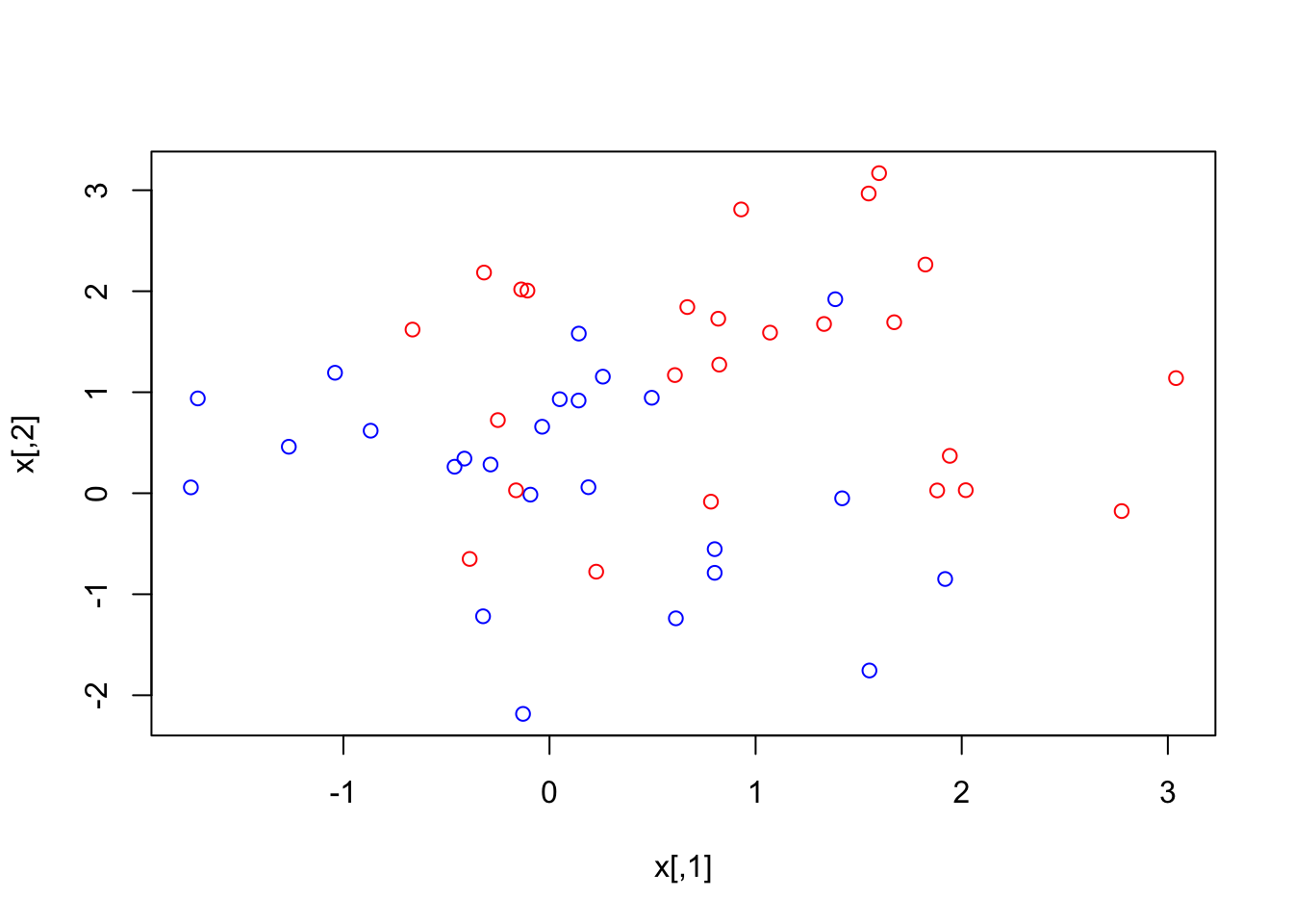

Data is clearly not linearly separable. There are two options:

Try to find a transformation of data that results in it being linearly separable and then fit a linear model (See Linear Basis Function Models at the end)
Fit a model that handles non-linearly separable data.

df <- data.frame(x = x, y = as.factor(y))
svcfit <- svm( y~., # Y as a function of all the other (so just x)
               data = df, # Specify where the data comes from
               kernel = "linear", # Fit an SVC (linear kernel)
               cost = 10, # This is the cost of crossing the Margin
               scale = FALSE) # Should the variables be scaled?
plot(svcfit , df)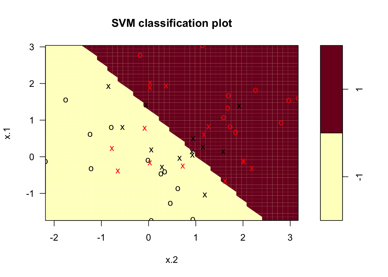

plot(x[,2], x[,1], col = (3 - y))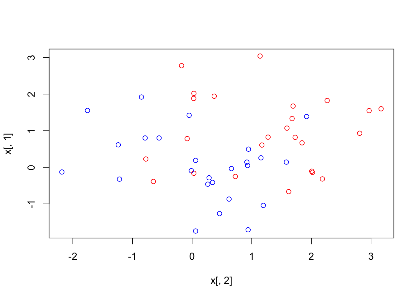

The light blue side corresponds to the $-1$ class and the pink one is the $1$ class. The support vectors are plotted as crosses, and the rest as circles. In the plot we can see 27 support vectors. We can also identify them by looking at the index of the svm object. We would also like to see what is in the summary of said object.

svcfit$index

##  [1]  1  2  5  6  7 10 12 14 17 19 21 22 24 26 27 29 30 31 35 37 38 39 40 42 45
## [26] 47 50

summary(svcfit)

## 
## Call:
## svm(formula = y ~ ., data = df, kernel = "linear", cost = 10, scale = FALSE)
## 
## 
## Parameters:
##    SVM-Type:  C-classification 
##  SVM-Kernel:  linear 
##        cost:  10 
## 
## Number of Support Vectors:  27
## 
##  ( 13 14 )
## 
## 
## Number of Classes:  2 
## 
## Levels: 
##  -1 1

Let’s now comare how changing the cost parameter changes the decision boundary.

svcfit2 <- svm( y~., # Y as a function of all the other (so just x)
               data = df, # Specify where the data comes from
               kernel = "linear", # Fit an SVC (linear kernel)
               cost = 0.1, # This is the cost of crossing the Margin
               scale = FALSE) # Should the variables be scaled?
plot(svcfit2 , df)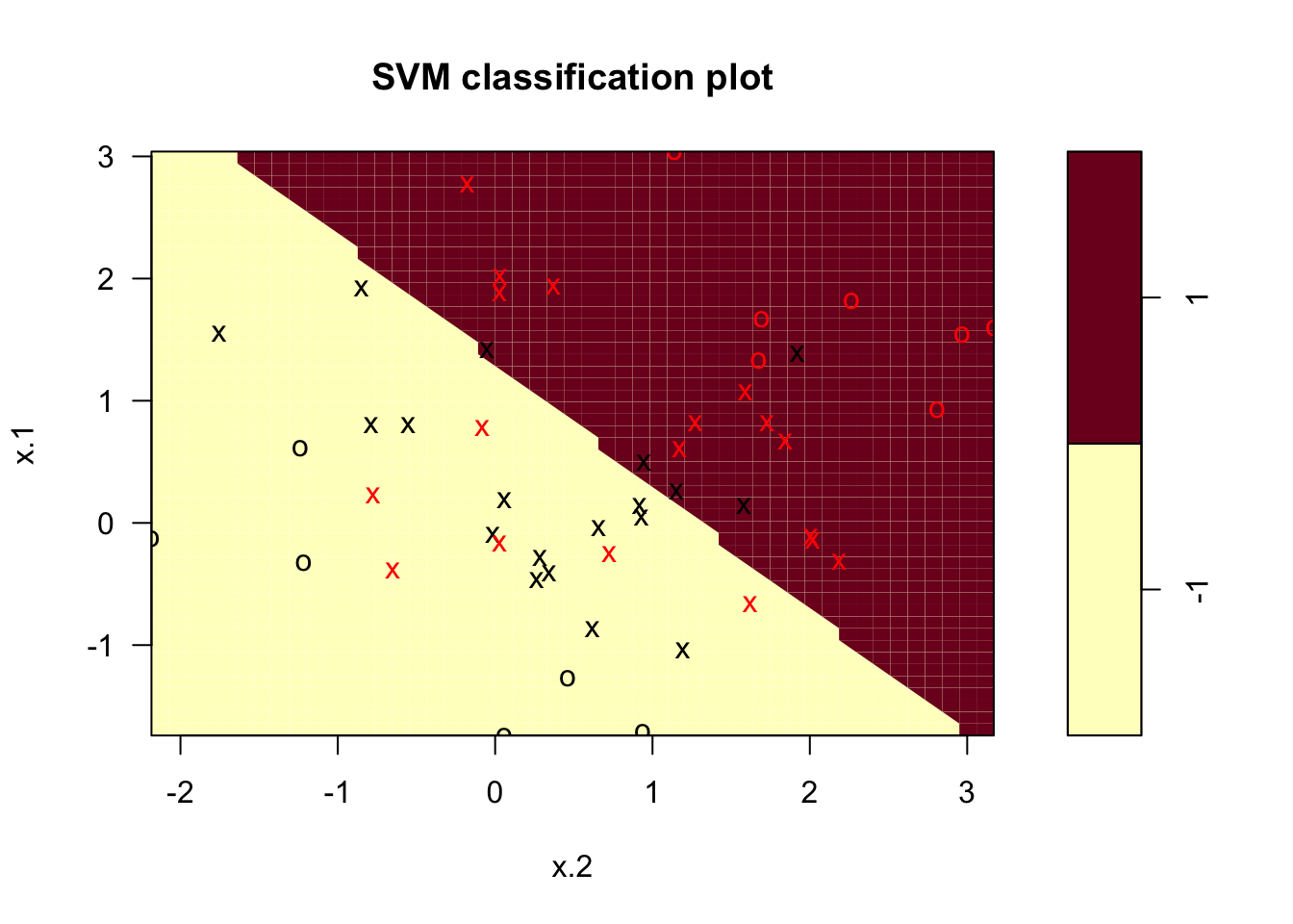

plot(x[,2], x[,1], col = (3 - y))

In this case the number of support vectors is expected to be higher, and as we can see it’s 37. This is due to the fact that the penalty for crossing the margin is relaxed. Now let’s look at what parameter results in the lowest possible loss via cross-validation:

tune.out <- tune(svm ,y~.,data = df ,kernel = "linear",
                 ranges = list(cost = c(0.001, 0.01, 0.1, 1,5,10,100)))
summary(tune.out)

## 
## Parameter tuning of 'svm':
## 
## - sampling method: 10-fold cross validation 
## 
## - best parameters:
##  cost
##   0.1
## 
## - best performance: 0.24 
## 
## - Detailed performance results:
##      cost error dispersion
## 1   0.001  0.66 0.09660918
## 2   0.010  0.64 0.12649111
## 3   0.100  0.24 0.20655911
## 4   1.000  0.28 0.16865481
## 5   5.000  0.28 0.16865481
## 6  10.000  0.28 0.16865481
## 7 100.000  0.28 0.16865481

This function stores the best iteration of the model which can be accessed in the following way:

best <- tune.out$best.model
summary(best)

## 
## Call:
## best.tune(method = svm, train.x = y ~ ., data = df, ranges = list(cost = c(0.001, 
##     0.01, 0.1, 1, 5, 10, 100)), kernel = "linear")
## 
## 
## Parameters:
##    SVM-Type:  C-classification 
##  SVM-Kernel:  linear 
##        cost:  0.1 
## 
## Number of Support Vectors:  38
## 
##  ( 19 19 )
## 
## 
## Number of Classes:  2 
## 
## Levels: 
##  -1 1

xtest <- matrix(rnorm(50*2) , ncol = 2)
ytest <- sample(c(-1,1), 50, rep = TRUE)
xtest[ytest == 1,] <- xtest[ytest == 1,] + 1
testdat <- data.frame(x = xtest, y = as.factor(ytest))

ypred <- predict(best ,testdat)
table(predict = ypred , truth = testdat$y )

##        truth
## predict -1  1
##      -1 20 12
##      1   3 15

Now let’s see what would happen if the data was linearly separable.

x[y == 1,] <- x[y == 1,] + 4
plot(x, col = (y + 5)/2, pch = 19)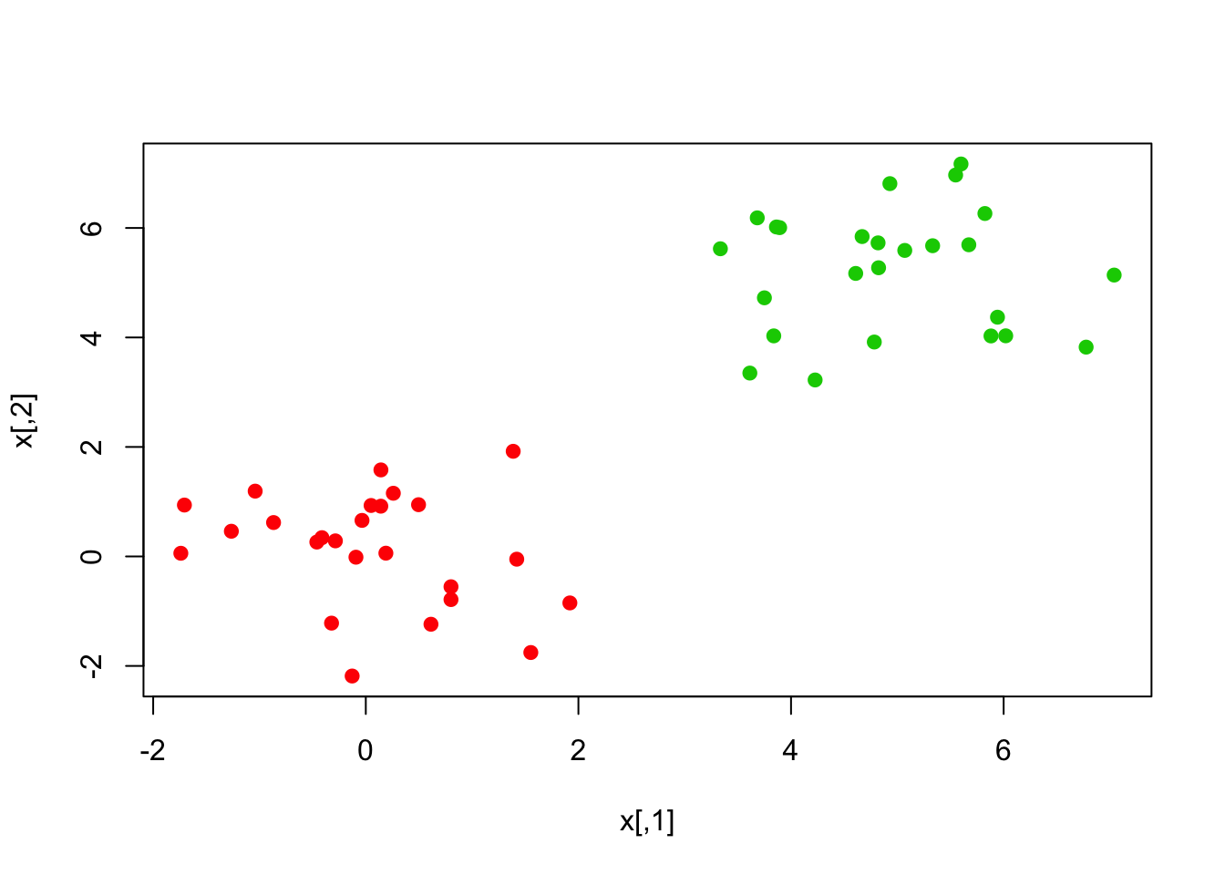

df2 <- data.frame(x = x, y = as.factor(y))
svcfit_new <- svm(y~., data = df2, kernel = "linear", cost = 1e5)
summary(svcfit_new)

## 
## Call:
## svm(formula = y ~ ., data = df2, kernel = "linear", cost = 100000)
## 
## 
## Parameters:
##    SVM-Type:  C-classification 
##  SVM-Kernel:  linear 
##        cost:  100000 
## 
## Number of Support Vectors:  2
## 
##  ( 1 1 )
## 
## 
## Number of Classes:  2 
## 
## Levels: 
##  -1 1

plot(svcfit_new, df2)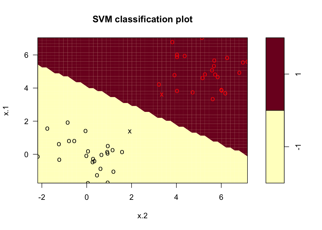

Let’s try a smaller value of cost since this might not be very good at performing on test data.

svcfit_new2 <- svm(y~., data = df2, kernel = "linear", cost = 1)
summary(svcfit_new2)

## 
## Call:
## svm(formula = y ~ ., data = df2, kernel = "linear", cost = 1)
## 
## 
## Parameters:
##    SVM-Type:  C-classification 
##  SVM-Kernel:  linear 
##        cost:  1 
## 
## Number of Support Vectors:  4
## 
##  ( 2 2 )
## 
## 
## Number of Classes:  2 
## 
## Levels: 
##  -1 1

plot(svcfit_new2, df2)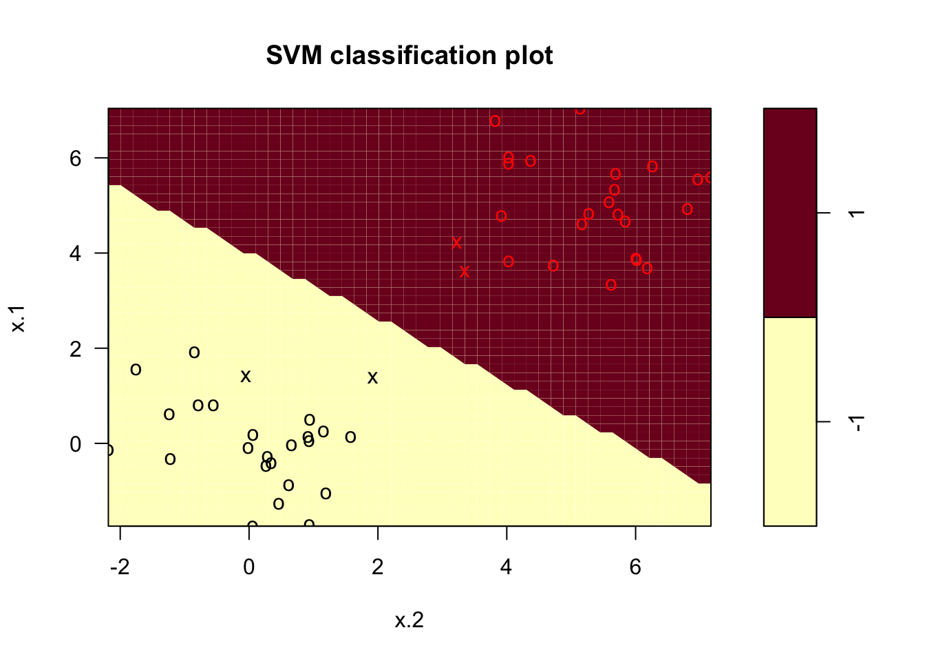

The decision boundary was linear as we expected, given that we specified it to be linear. Let’s see what happens if we remove that constraint.

svmfit <- svm( y~., # Y as a function of all the other (so just x)
               data = df, # Specify where the data comes from
               cost = 10, # This is the cost of crossing the Margin
               kernel = "polynomial",
               scale = FALSE) # Should the variables be scaled?
plot(svmfit , df)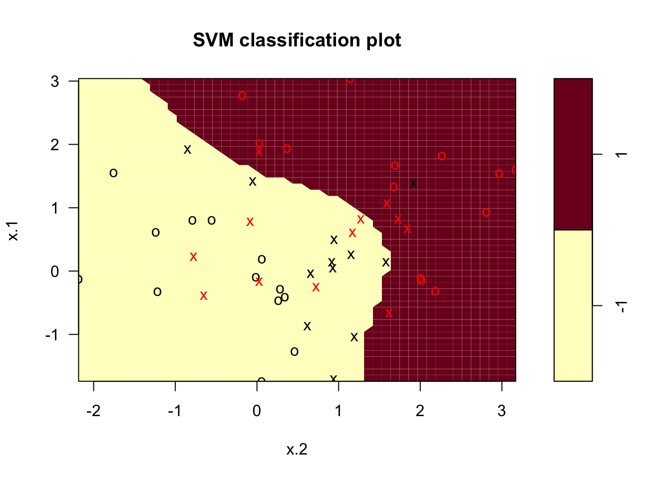

Question 3

Question:

Consider the support vector classifier with the Lagrangian \[ L(\beta,\beta_0,\xi,\lambda,\mu) = \frac{1}{2} \beta^T\beta + C\sum_{i=1}^n \xi_i - \sum_{i=1}^n\lambda_i\left[y_i(x_i^T\beta + \beta_0)-1 + \xi_i\right] - \sum_{i=1}^n \mu_i \xi_i \] Using the KKT equations, show that the optimal $\beta$ can be written as

\[ \beta = \sum_{i=1}^n \lambda_iy_i x_i. \]

Show that $\lambda$ solves \[\begin{align*} &\max_\lambda \sum_{i=1}^n\lambda_i - \frac{1}{2}\sum_{i=1}^n \sum_{j=1}^n y_iy_j\lambda_i\lambda_j x_i^Tx_j\\ &\text{Subject to:}\\ &\qquad 0\leq \lambda_i \leq C,\quad i=1,\ldots, n \\ &\qquad \sum_{i=1}^n \lambda_i y_i = 0. \end{align*}\] Argue that \[\begin{align*} \lambda_i = 0 & \Rightarrow y_i( \beta^T x_i + \beta_0) \geq 1 \\ \lambda_i = C & \Rightarrow y_i( \beta^T x_i + \beta_0) \leq 1 \\ 0 < \lambda_i < C & \Rightarrow y_i( \beta^T x_i + \beta_0) = 1. \end{align*}\]

Solution:

The KKT conditions say that we need to satisfy $\frac{\partial L}{\partial \beta_0} = 0$. This implies \[ - \sum_{i=1}^n \lambda_i y_i \beta_0 = 0 \] which is satisfied if $\sum_{i=1}^n \lambda_iy_i=0$.

We also need $\nabla_\beta L = 0$. Doing the derivative, this condition is \[ \beta -\sum_{i=1}^n\lambda_i y_i x_i = 0 \] or, equivalently, $\beta =\sum_{i=1}^n\lambda_i y_i x_i$.

We also need $\nabla_\xi L =0$ which holds when \[ C1 - \lambda - \mu = 0, \] where $1$ is the vector of 1s. This implies $\mu_i = C - \lambda_i$. Combining this with the condition that $\mu_i \geq 0$ and $\lambda_i \geq 0$, it follows that $0 \leq \lambda_i \leq C$.

Substituting all of this into the Lagrangian we get \[\begin{align*} L &= \frac{1}{2} \left(\sum_{i=1}^n\lambda_i y_i x_i\right)^T\left(\sum_{j=1}^n\lambda_j y_j x_j\right) + C\sum_{i=1}^n \xi_i - \sum_{i=1}^n\lambda_i\left[y_i(x_i^T\left(\sum_{j=1}^n\lambda_j y_j x_j\right) + \beta_0)-1 + \xi_i\right] - \sum_{i=1}^n (C-\lambda_i) \xi_i \\ &=\frac{1}{2}\sum_{i=1}^n \sum_{j=1}^n\lambda_i\lambda_j y_iy_j x_i^Tx_j + C \sum_{i=1}^n \xi_i - \sum_{i=1}^n\sum_{j=1}^n \lambda_i\lambda_jy_iy_j x_i^Tx_j - \beta_0\sum_{i=1}^n \lambda_i y_i + \sum_{i=1}^n\lambda_i - \sum_{i=1}^n\lambda_i\xi_i - C\sum_{i=1}^n \xi_i + \sum_{i=1}^n \lambda_i\xi_i \\ &=\sum_{i=1}^n \lambda_i - \frac{1}{2}\sum_{i=1}^n \sum_{j=1}^n\lambda_i\lambda_j y_iy_j x_i^Tx_j . \end{align*}\]

By strong duality, we want to find the $\lambda$ that maximizes this Lagrangian under the constraints, which gives \[\begin{align*} &\max_\lambda \sum_{i=1}^n\lambda_i - \frac{1}{2}\sum_{i=1}^n \sum_{j=1}^n y_iy_j\lambda_i\lambda_j x_i^Tx_j\\ &\text{Subject to:}\\ &\qquad 0\leq \lambda_i \leq C,\quad i=1,\ldots, n \\ &\qquad \sum_{i=1}^n \lambda_i y_i = 0. \end{align*}\]

Finally, by complementatry slackness we know that $\lambda_i[y_i(\beta_0 + \beta^Tx_i ) - 1 + \xi_i] = 0$ and $\xi_i(C-\lambda_i)=0$. When $\lambda_i=0$, that means that $C \xi_i=0$ which implies $\xi_i=0$, which means that the observation is on the correct side of the margin. When $\lambda_i=C$, that means that $\xi_i\geq 0$ and hence, we are on teh wrong side of the margin. If $0<\lambda < C$, the second complementary slackness condition gives $\xi=0$, while the first gives $[y_i(\beta_0 + \beta^Tx_i ) = 1$.

Linear Basis Function Models

Again with thanks to Alex Stringer

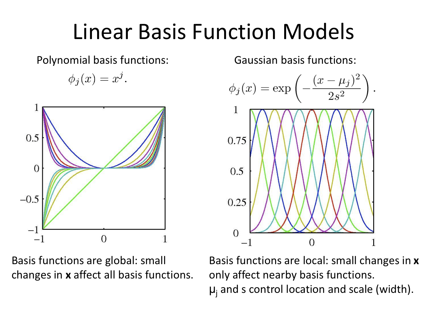
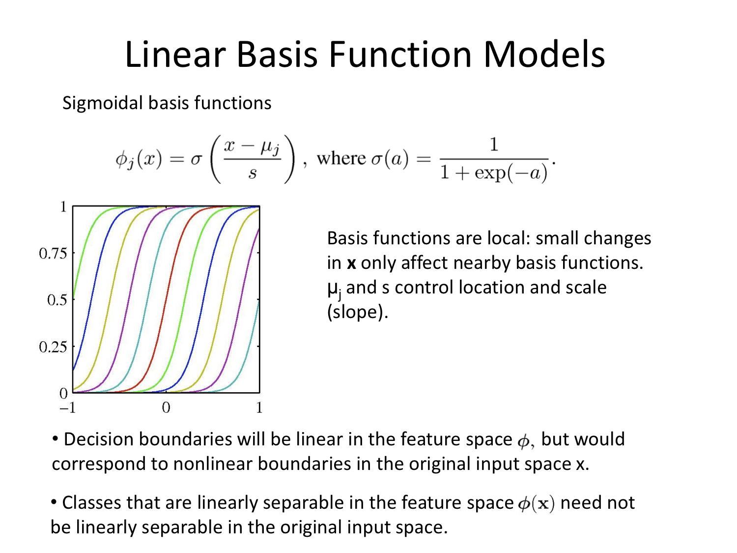
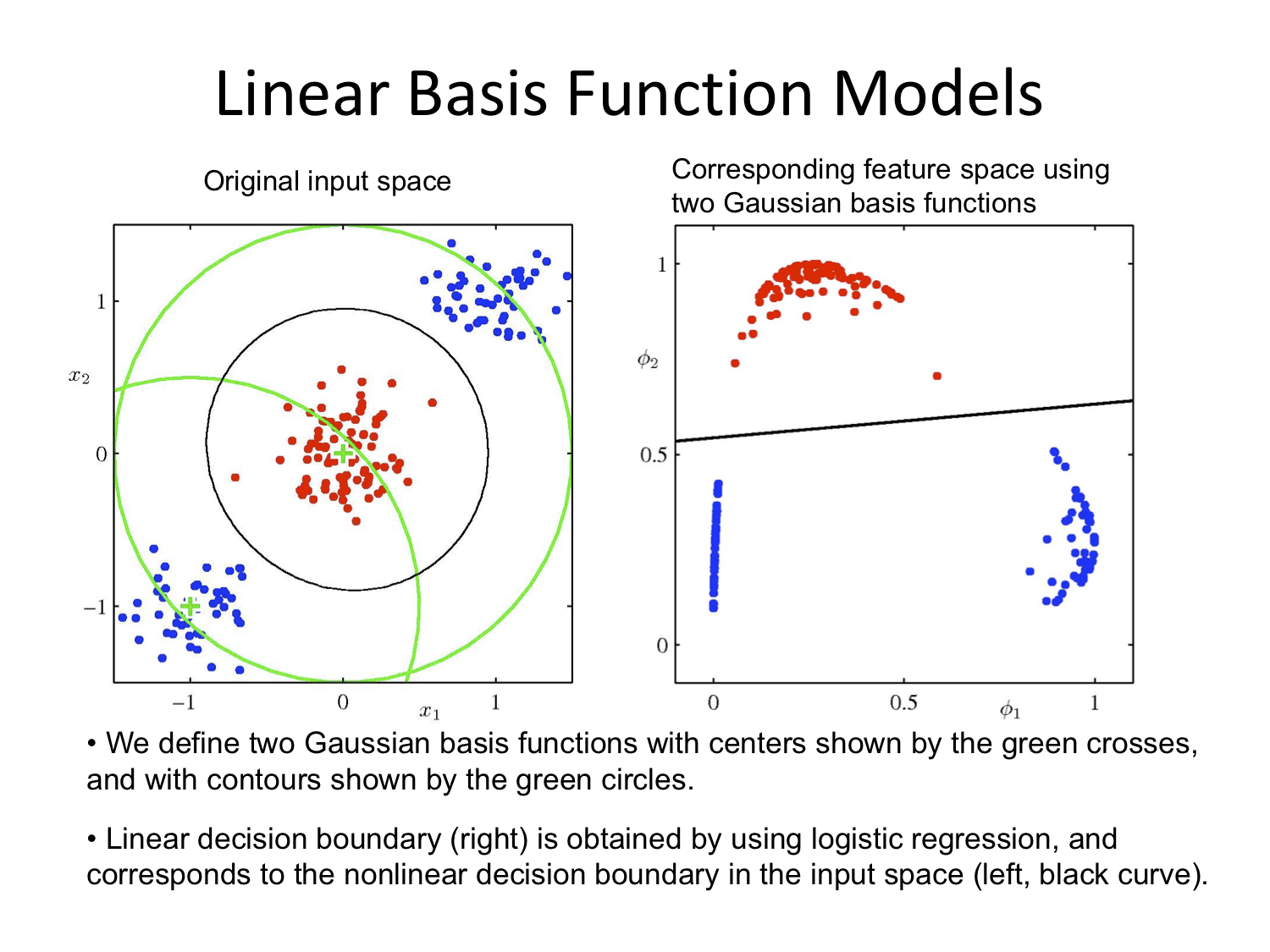
Week 10

Question 2

par(xpd = NA)
plot(NA, NA, type = "n", xlim = c(-2, 2), ylim = c(-3, 3), xlab = "X1", ylab = "X2")
# X2 < 1
lines(x = c(-2, 2), y = c(1, 1))
# X1 < 1 with X2 < 1
lines(x = c(1, 1), y = c(-3, 1))
text(x = (-2 + 1)/2, y = -1, labels = c(-1.8))
text(x = 1.5, y = -1, labels = c(0.63))
# X2 < 2 with X2 >= 1
lines(x = c(-2, 2), y = c(2, 2))
text(x = 0, y = 2.5, labels = c(2.49))
# X1 < 0 with X2<2 and X2>=1
lines(x = c(0, 0), y = c(1, 2))
text(x = -1, y = 1.5, labels = c(-1.06))
text(x = 1, y = 1.5, labels = c(0.21))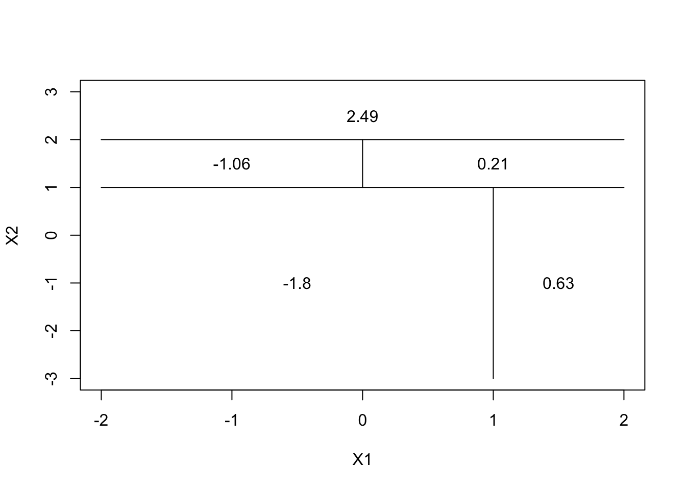

Question 3

p <- seq(0, 1, by = 0.01)
gini <- p * (1 - p) * 2
CE <- -(p * log(p) + (1 - p) * log(1 - p))
Class.Err <- 1 - pmax(p, 1 - p)
df <- tibble(p = p, gini = gini, CE = CE, ClassError = Class.Err)
ggplot(data = df, mapping = aes(x = p)) +
    geom_point(mapping = aes(x = p, y = gini), color = "red", shape = "G") +
    geom_point(mapping = aes(x = p, y = CE), color = "blue", shape = "C") +
    geom_point(mapping = aes(x = p, y = Class.Err), color = "green", shape = "E")

## Warning: Removed 2 rows containing missing values (geom_point).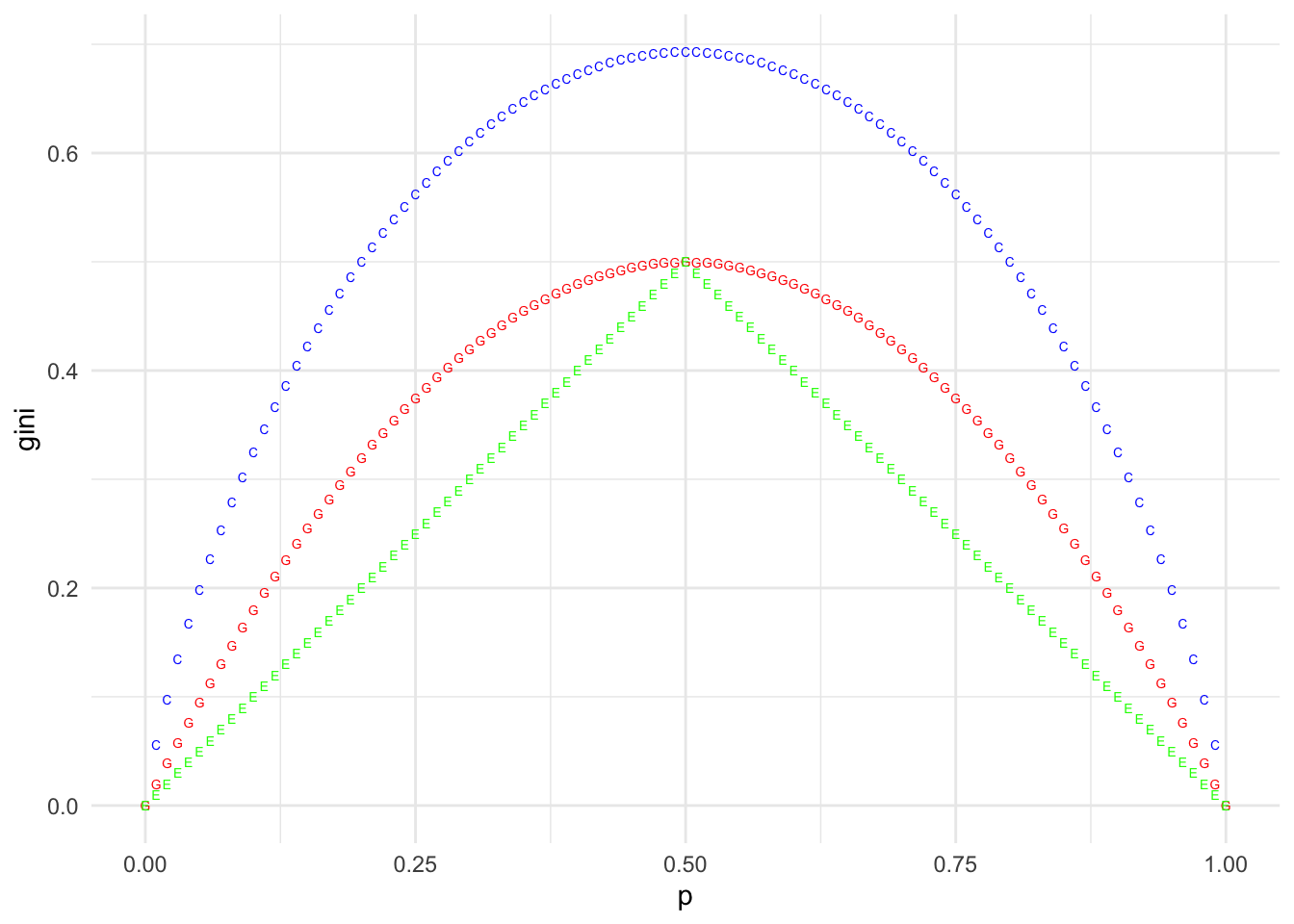

Additional Material

This week we talked about Decision Tree algorithms, boosting, bagging, and model explainability.

Algorithms in Practice

If you are interested more in how we use those algorithms in practice, implementations, parameters etc.

My code in Python using LightGBM package can be found here. ** note that the runtime of the kernel is just shy of 6 hours on the server **

What you mind find interesting in particular are the parameters for the Tree Models:

n_estimators=10000; number of boosting iterations (so 10000 weak models)
learning_rate=0.02; shrinkage rate (what should be the “strength” of each model)
num_leaves=34; max number of leaves in one tree
colsample_bytree=0.9497036; fraction of features to be considered for each tree note that this is very far from $\sqrt{p}$ since p was around 1000, this could be ~3% not 95%
subsample=0.8715623; fraction of data in each bag (I am not using the full dataset size at each step)
max_depth=8; max deapth of each tree
reg_alpha=0.041545473; L1 regularization parameter
reg_lambda=0.0735294; L2 regularization parameter
min_split_gain=0.0222415; minimum loss decrease for a split to be kept
min_child_weight=39.3259775; minimum amount of data in each rectangle

If you are interested in how the parameter values were found I highly recommend taking a deeper dive into Bayesian Optimization.

Let’s now see how we can use the xgboost package in R to analyze some data. I will be using the wine classification challenge from UCI. link

rm(list = ls()) 
# Load the data
df <- read_csv("https://archive.ics.uci.edu/ml/machine-learning-databases/wine/wine.data",
         col_names = c("Class",
                      "Alcohol",
                      "Malic Acid",
                      "Ash",
                      "Alcalinity of ash",
                      "Magnesium",
                      "Total phenols",
                      "Flavanoids",
                      "Nonflavanoid phenols",
                      "Proanthocyanins",
                      "Color intensity",
                      "Hue",
                      "OD280/OD315 of diluted wines",
                      "Proline"))

## Parsed with column specification:
## cols(
##   Class = col_double(),
##   Alcohol = col_double(),
##   `Malic Acid` = col_double(),
##   Ash = col_double(),
##   `Alcalinity of ash` = col_double(),
##   Magnesium = col_double(),
##   `Total phenols` = col_double(),
##   Flavanoids = col_double(),
##   `Nonflavanoid phenols` = col_double(),
##   Proanthocyanins = col_double(),
##   `Color intensity` = col_double(),
##   Hue = col_double(),
##   `OD280/OD315 of diluted wines` = col_double(),
##   Proline = col_double()
## )

# Look at the class distribution
ggplot(data = df, aes(x = Class)) +
    geom_bar()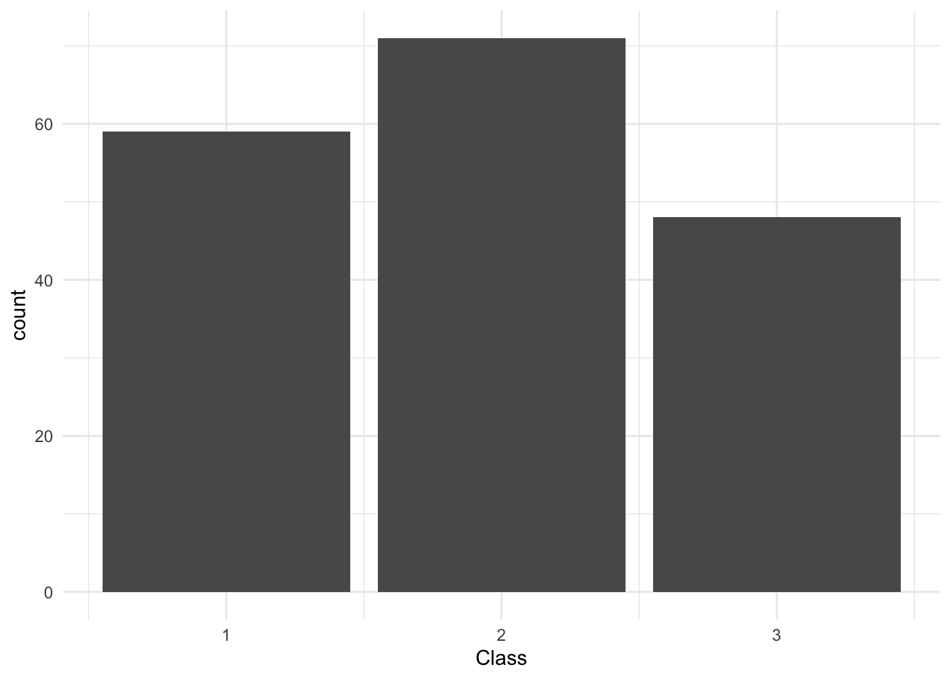

# We see that the classes are imbalanced but that's fine.
# I will try to create a new class feature to make it a binary classification
df2 <- df %>% mutate(Hue_class = if_else(Hue < 1, 0, 1)) %>% dplyr::select(-Hue)

## mutate: new variable 'Hue_class' with 2 unique values and 0% NA

df2 %>% group_by(Hue_class) %>% summarise(n = n())

## group_by: one grouping variable (Hue_class)

## summarise: now 2 rows and 2 columns, ungrouped

## # A tibble: 2 x 2
##   Hue_class     n
##       <dbl> <int>
## 1         0    94
## 2         1    84

# Now the classes are closer to balanced and we can drop the class variable.

Our task is now to predict wether Hue will be lower or higher than 1 for a given wine. Hue_Class is our new response variable. Now I will walk you through setting up the data to use xgboost. We need to convert our dataset into a Model Matrix.

# Create a model matrix object, this is usually a way of dealing with data
# for xgboost.
MM <- model.matrix(df2, object = Hue_class ~. - 1)

# Create a training set
indexes = sample(1:nrow(df2), size = 0.7*nrow(df2),replace = FALSE)
MM_train <- MM[indexes,]
MM_test <- MM[-indexes,]

testset <- as.tibble(MM_test)

# Create the DMatrix type for xgboost.
dtrain <- xgb.DMatrix(data = MM_train, label = df2[indexes,]$Hue_class)

# Fit the model
xgb_model <- xgboost(data = dtrain,
        max.depth = 3,
        eta = 0.1,
        nrounds = 30,
        verbose = 1,
        objective = "binary:logistic"
        )

## [1]  train-error:0.169355 
## [2]  train-error:0.145161 
## [3]  train-error:0.145161 
## [4]  train-error:0.145161 
## [5]  train-error:0.145161 
## [6]  train-error:0.161290 
## [7]  train-error:0.169355 
## [8]  train-error:0.169355 
## [9]  train-error:0.161290 
## [10] train-error:0.169355 
## [11] train-error:0.153226 
## [12] train-error:0.145161 
## [13] train-error:0.153226 
## [14] train-error:0.153226 
## [15] train-error:0.153226 
## [16] train-error:0.120968 
## [17] train-error:0.112903 
## [18] train-error:0.112903 
## [19] train-error:0.112903 
## [20] train-error:0.112903 
## [21] train-error:0.096774 
## [22] train-error:0.096774 
## [23] train-error:0.088710 
## [24] train-error:0.088710 
## [25] train-error:0.056452 
## [26] train-error:0.056452 
## [27] train-error:0.064516 
## [28] train-error:0.048387 
## [29] train-error:0.048387 
## [30] train-error:0.048387

# Predict and test
predictions <- predict(xgb_model, MM_test)
predictions

##  [1] 0.50780773 0.79457676 0.90337294 0.62081563 0.82798505 0.80860537
##  [7] 0.64622140 0.79126465 0.84566784 0.87311476 0.52419418 0.30696177
## [13] 0.62619990 0.55615032 0.72600758 0.57412136 0.80958211 0.67523229
## [19] 0.80958211 0.59415364 0.74965417 0.58946824 0.78325748 0.79056698
## [25] 0.81800616 0.52827030 0.70411801 0.78714371 0.74454254 0.74708617
## [31] 0.60665971 0.62924165 0.48607311 0.52549106 0.65133184 0.75830501
## [37] 0.22120035 0.68859750 0.46560755 0.60352784 0.64660317 0.38752475
## [43] 0.71704257 0.64633924 0.06538267 0.04596485 0.05368504 0.04596485
## [49] 0.05004754 0.05004754 0.04790421 0.04153613 0.07550301 0.04153613

# Plot the ROC for our tree
roc <- roc(response = df2[-indexes,]$Hue_class, predictions)

## Setting levels: control = 0, case = 1

## Setting direction: controls < cases

plot(roc)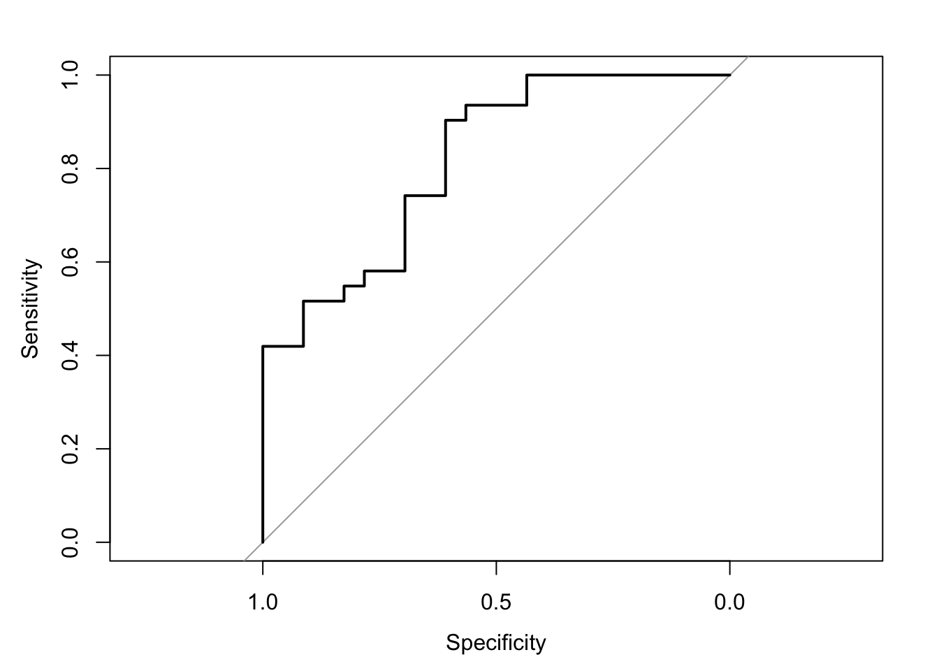

print(roc$auc)

## Area under the curve: 0.8163

# This is not horrible!
# Let's see what our trees actually look like:
xgb.plot.tree(model = xgb_model, trees = 0)

xgb.plot.tree(model = xgb_model, trees = 1)

STA314 Materials

Michal Malyska

Preamble

Resources

Library Load

Week 1

Week 2

Week 3

Question 2

Task : Use this algorithm to make a 4 clustering of the data set in question2.RData. Comment on the clustering.

Question 3

Question 4

Week 4

Lab 2

R for data science chapter 25: Many Models

Week 5

Principal Component Analysis

Motivation:

Procedure:

Lab 1: PCA

Lab 3: PCA and Clustering

Question 3:

Question:

Solution:

Question 4

Question:

Solution:

i)

ii)

iii)

Questions from the tutorial:

Spectral Decomposition explanation

Why is variance-covariance positive semi-definite? i.e. why is \(S = Q \Lambda Q^T\)

Week 6

Week 7

Lab 6

Question 1

Question

Question 2

Question

Solution

Week 8

Week 9

Lab 5

Question 3

Question:

Solution:

Linear Basis Function Models

Week 10

Question 2

Question 3

Additional Material

Algorithms in Practice